In this project, we will use what we've learned about deep neural networks and convolutional neural networks to classify traffic signs. We will train and validate a model so it can classify traffic sign images using the German Traffic Sign Dataset. After the model is trained, we will then try out our model on images of German traffic signs that we find on the web.
The following Ipython notebook was used as started point for our own implementation.
The main files of this project are:
- the Ipython notebook with the code
- the code exported as an html file
- this detailed documentation
The goals / steps of this project are the following:
- Load the German Traffic Sign data set
- Explore, summarize and visualize the data set
- Design, train and test a model architecture
- Use the model to make predictions on new images
- Analyze the softmax probabilities of the new images
- Summarize the results in this documentation
This lab requires:
The lab environment can be created with CarND Term1 Starter Kit. Click here for the details. We used Docker and all worked perfectly.
-
Download the data set. This is a pickled dataset in which images were resized to 32x32. It contains a training, validation and test set.
-
Clone the project, which contains the Ipython notebook and the writeup template.
git clone https://github.com/udacity/CarND-Traffic-Sign-Classifier-Project
cd CarND-Traffic-Sign-Classifier-Project
jupyter notebook Traffic_Sign_Classifier.ipynbWe used the pandas library to calculate summary statistics of the traffic signs data set:
- The size of training set is 34799
- The size of the validation set is 4410
- The size of test set is 12630
- The shape of a traffic sign image is (32,32,3)
- The number of unique classes/labels in the data set is 43 which are the following:
| Class Id | Sign Name |
|---|---|
| 0 | Speed limit (20km/h) |
| 1 | Speed limit (30km/h) |
| 2 | Speed limit (50km/h) |
| 3 | Speed limit (60km/h) |
| 4 | Speed limit (70km/h) |
| 5 | Speed limit (80km/h) |
| 6 | End of speed limit (80km/h) |
| 7 | Speed limit (100km/h) |
| 8 | Speed limit (120km/h) |
| 9 | No passing |
| 10 | No passing for vehicles over 3.5 metric tons |
| 11 | Right-of-way at the next intersection |
| 12 | Priority road |
| 13 | Yield |
| 14 | Stop |
| 15 | No vehicles |
| 16 | Vehicles over 3.5 metric tons prohibited |
| 17 | No entry |
| 18 | General caution |
| 19 | Dangerous curve to the left |
| 20 | Dangerous curve to the right |
| 21 | Double curve |
| 22 | Bumpy road |
| 23 | Slippery road |
| 24 | Road narrows on the right |
| 25 | Road work |
| 26 | Traffic signals |
| 27 | Pedestrians |
| 28 | Children crossing |
| 29 | Bicycles crossing |
| 30 | Beware of ice/snow |
| 31 | Wild animals crossing |
| 32 | End of all speed and passing limits |
| 33 | Turn right ahead |
| 34 | Turn left ahead |
| 35 | Ahead only |
| 36 | Go straight or right |
| 37 | Go straight or left |
| 38 | Keep right |
| 39 | Keep left |
| 40 | Roundabout mandatory |
| 41 | End of no passing |
| 42 | End of no passing by vehicles over 3.5 metric ... |
We have tested if the training, validation and test sets contains samples of each class which is necessary because we must train, validate and test with samples from each class. In this case, samples are correctly distributed over all sets.
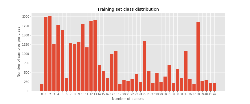
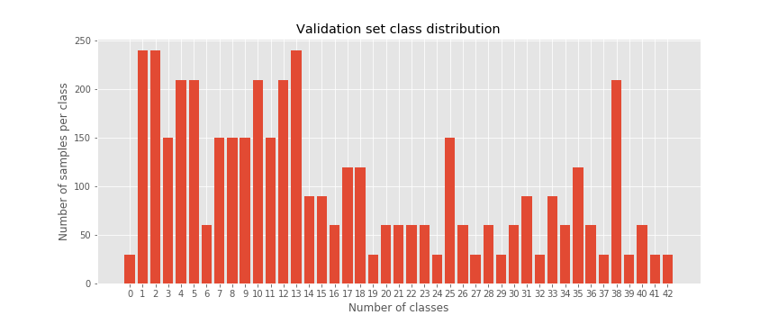
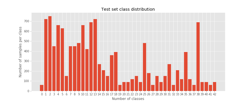
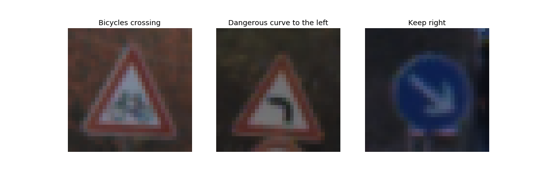
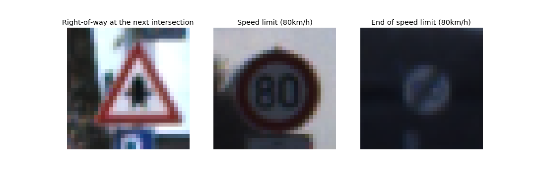
We analyzed the class distribution in each split of the data set. At the same time we randomly plot a few examples of each split alongside its label. We will firstly plot several bar charts showing the class distribution on the training, validation and test sets.
Regarding the per-class occurrences in each set we noticed that we are facing a quite imbalanced data set. However validation and test sets are more balanced. The best way to solve this problem is using data augmentation techniques.
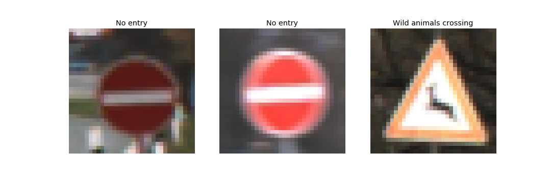
Next we will plot 3 random samples from each set.
We observe that the samples may be different from each other taking into account changes in illumination, contrast and camera viewing angle. Due to, we are facing a quite complex data set.
In this section we will describe the techniques were chosen in order to preprocess our input data.
We used the following techniques implemented and applied in the same order as their are listed:
- conversion from RGB to grayscale
- image scaling
- local image equalization with disk filter or global image equalization
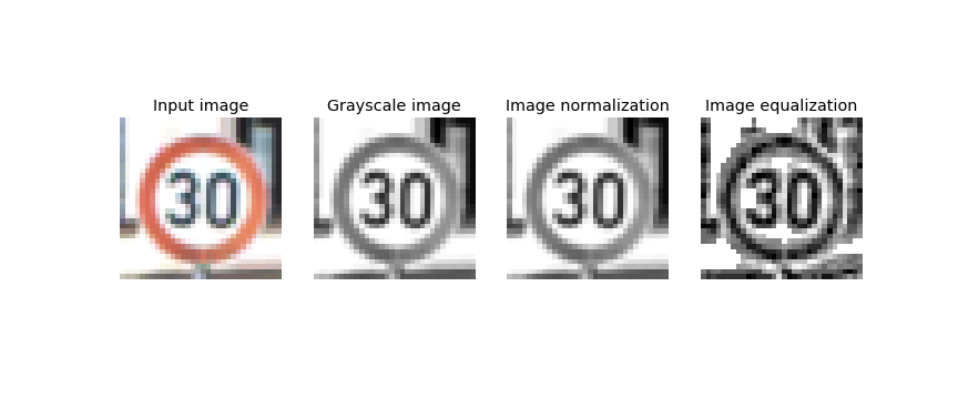
As a first step, we decided to convert the images to grayscale because state-of-the-art works prove that color infomraciton in the case of traffic sign classificacion didn't make the difference. We then used image scaling in order to standardize the range of independent variables or features of data. Finally we applied a global image equalization which worked worst than local image equalization with disk filter which obtained better results. In our case, image normalization didn't worked well. When image normalization was appllied the model converge slower to the solution.
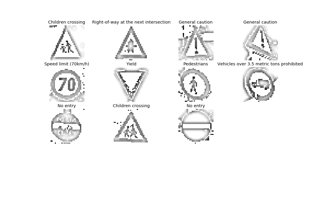
Here are several examples of traffic sign images before and after applying the preprocessing step.
In this section we will describe what our final model architecture looks like (model type, layers, layer sizes, connectivity, etc.) We will include a diagram and/or table describing the final model.
My final model consisted of the following layers:
| Layer | Description |
|---|---|
| Input | 32x32x1 grayscale image |
| Convolution 3x3 | 1x1 stride, valid padding, outputs 30x30x16 |
| RELU | |
| Max pooling | 2x2 stride, valid padding outputs 15x15x16 |
| Convolution 6x6 | 1x1 stride, valid padding, outputs 10x10x32 |
| RELU | |
| Max pooling | 2x2 stride, valid padding, outputs 5x5x32 |
| Flatten | outputs 800 |
| Fully connected | outputs 512 |
| RELU | |
| Dropout | keep_prob= 0.4 |
| Fully connected | outputs 256 |
| RELU | |
| Dropout | keep_prob= 0.4 |
| Fully connected | outputs 43 |
| Logits |
In this section we will describe how we trained our model (type of optimizer, the batch size, number of epochs, learning rate, etc.)
To train my model we used softmax corss entropy with one-hot encoded labels. Moreover, Adam optimizer was used in order to improve the gradient descent. Training was done on a Tesla K40 GPU with the following parameters:
- batch size = 256
- training epochs = 32
- learning rate = 0.001
During the 32 epochs we observed that training and validation losses converged steadily and constantly to the minimum global. At the same time, training and validation accuracies where increasing. We noticed that the best validation loss was achieved during epoch 28 where the training accuracy was 0.998 (almost 1.0), validation accuracy was 0.986, validation loss was 0.134 and finally training loss 0.007. With this model we achieved a 0.953 accuracy value using the test set.
In order to get to this solution we test with different models varying the number of layers, convolution kernels, max pooling, strides, dropout values and also number of neurons in the fully connected layers. Moreover, we tested different learning rates.
Our model is overfitting over the training set, nevertheless the validation loss is mantained higher than the training one. The final test would be using new input data from internet. There we will see if our model generalize well using new input data.
The first architecture we used was the LeNet-5 architecture. With this approach we obtained lower validation accuracies and model get stucked after only a few epochs. Due to, we increased the complexity of our architecture to obtain better results. This process was totally based on an exhaustive experimentation. With these changes we avoid underfitting due to the low model complexity, and we avoided overfitting due to the lack of data (by using dropout). We also improved the results increasing the batch size to 256. Training process was quite faster and results were better.
My final model results were:
- training set accuracy of 0.998
- validation set accuracy of 0.969
- test set accuracy of 0.953
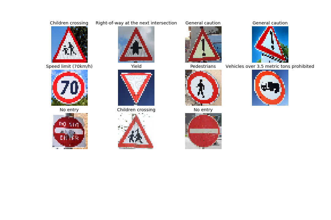
In this section we will choose five German traffic signs founded on the web in order to test our model with new input data. By this way, we will know if our model generalize well over new input data. For each image, we will discuss what quality or qualities might be difficult to classify.
Here are the German traffic signs that I found on the web:
The same images after the preprocessing stage:
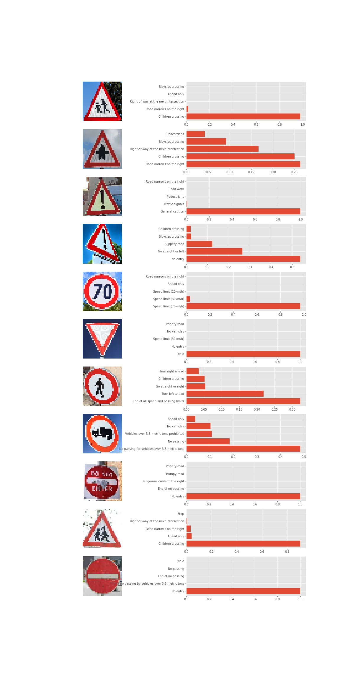
An finally the obtained probabilities:
As we observed, the model was able to classify correctly 8 images of 11 which is a quite good result. The misclassified images are because of the lack of data. We noticed that the presence of a different sight angle in the image will conduct to a misclassification.
Looking at the probabilities we are able to see what classes the model is wrong with.

