Application of U-Net in Lung Segmentation
This Implementation Achived 97% accuracy in Lung Segmentation with U-Net
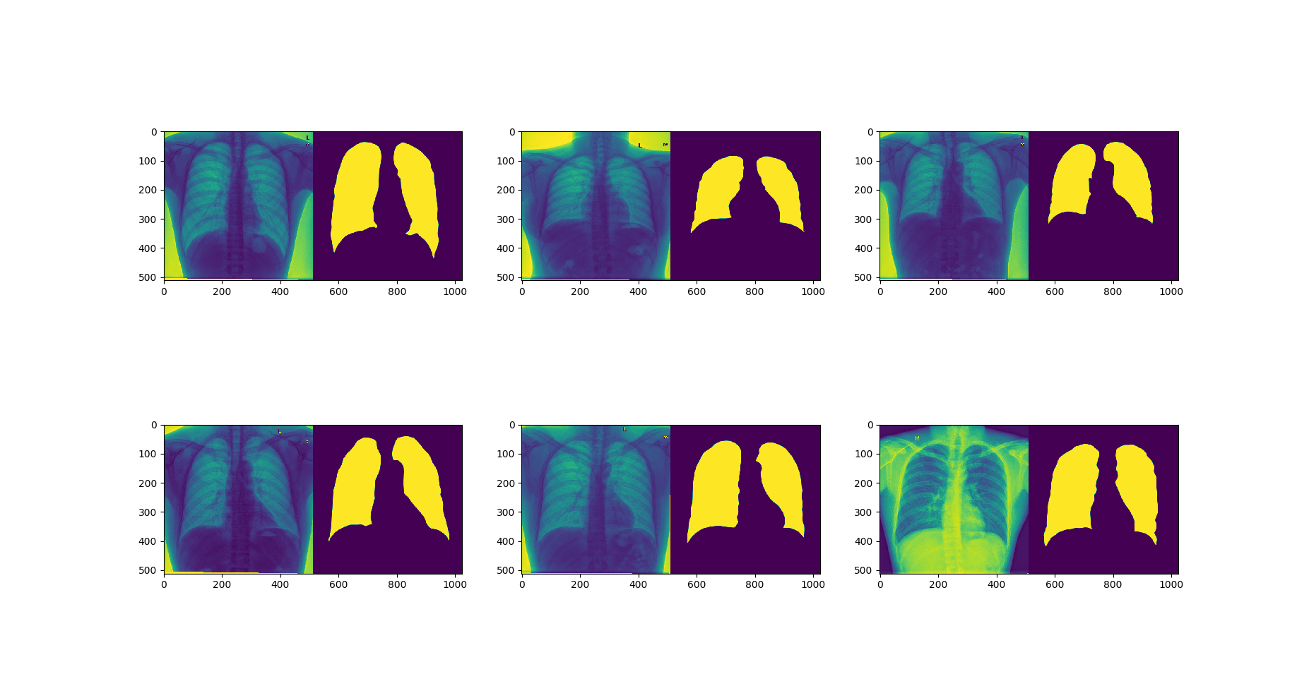
Download Dataset from Chest Xray Masks and Labels Pulmonary Chest X-Ray Defect Detection
  /data
    /data/Lung Segmentation
      /data/Lung Segmentation/CXR_Png
      /data/Lung Segmentation/masks
Writers: Olaf Ronneberger, Philipp Fischer, and Thomas Brox
Medical Image Computing and Computer-Assisted Intervention (MICCAI), Springer, LNCS, Vol.9351: 234--241, 2015, available at https://arxiv.org/pdf/1505.04597.pdf
U-Net is a convolutional neural network architecture for fast and precise segmentation of images.
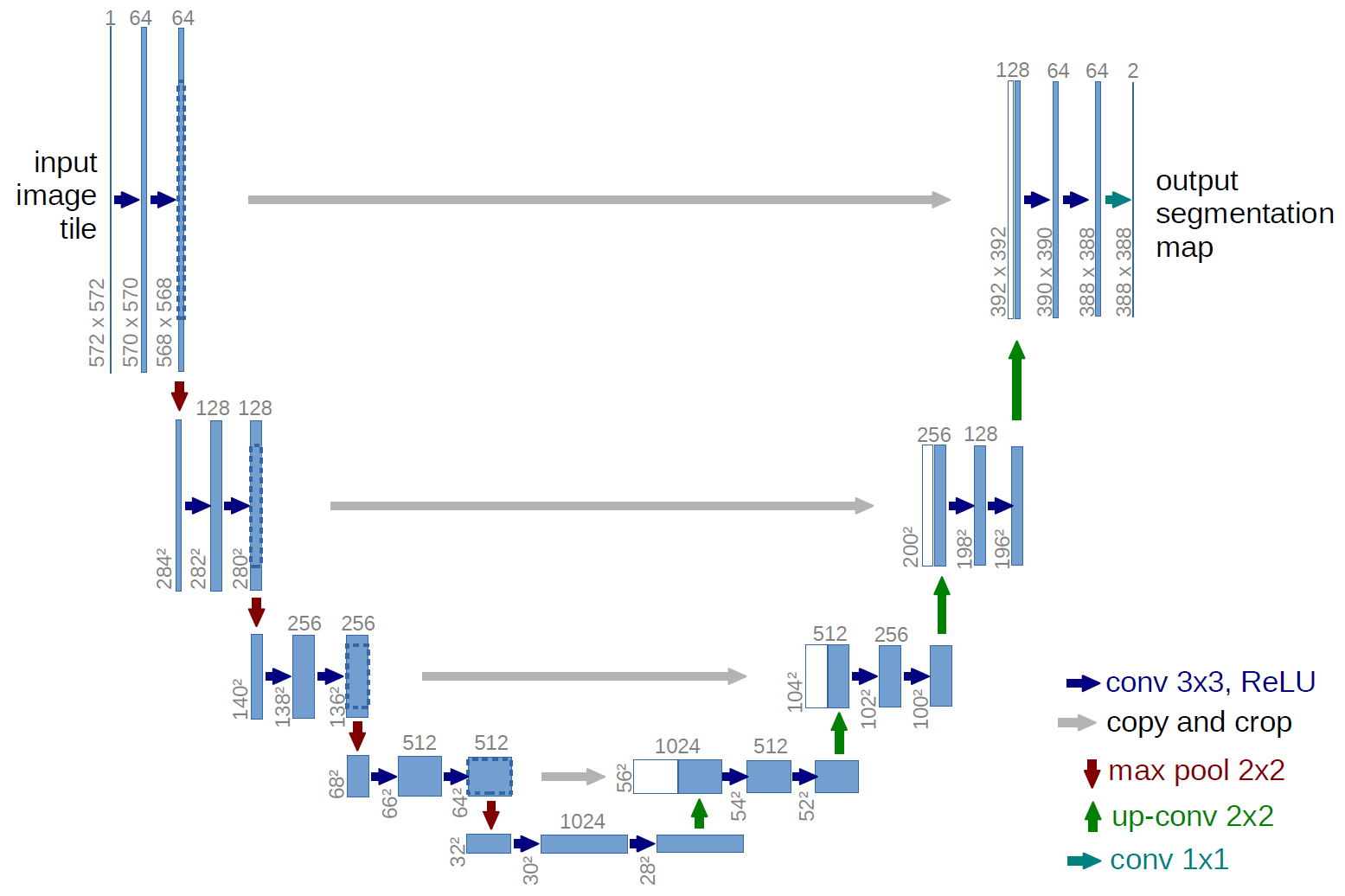
U-net architecture (example for 32x32 pixels in the lowest resolution). Each blue box corresponds to a multi-channel feature map. The number of channels is denoted on top of the box. The x-y-size is provided at the lower left edge of the box. White boxes represent copied feature maps. The arrows denote the different operations.
Note that there is no dense layer.So images of different sizes can be used as input.
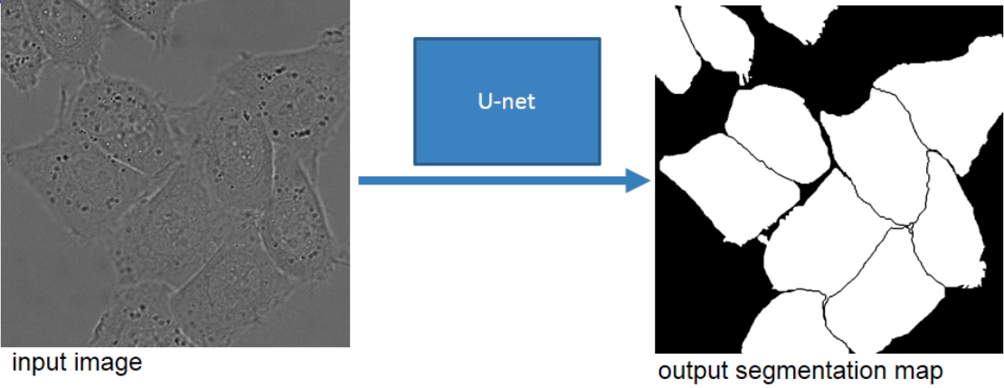
The U-Net combines the location information from the downsampling with the contextual information in the upsampling path to finally obtain a general information combining localisation and context, which is necessary to predict a good segmentation map.
It consists of the repeated application of :
- Two 3x3 convolutions (unpadded convolutions)
- Followed by a ReLU (Rectified Linear Unit) and Batch Normalization
- A 2x2 max pooling operation with stride 2 for downsampling.
Sequence of up-convolutions and concatenation(skip-connection) with high-resolution features from contracting path :
- 2x2 convolution ("up-convolution") that halves the number of feature channels
- A concatenation with the correspondingly cropped feature map from the contracting path
- Two 3x3 convolutions
- Followed by a ReLU with Batch Normalization
At the final layer a 1x1 convolution is used to map each 64 componet feature vector to the desired number of classes.
- Very few annotated Very few annotated images available (approx. 30 per applications)
- Touching objects of the same class
- U-net learns segmentation in an end-to-end setting (beats the prior best method, a sliding-window CNN, with large margin.)
- excessive data augmentation by applying elastic deformations which used to be the most common variation in tissue and realistic deformations can be simulated efficiently.
- Ensure Separation of Touching Objects
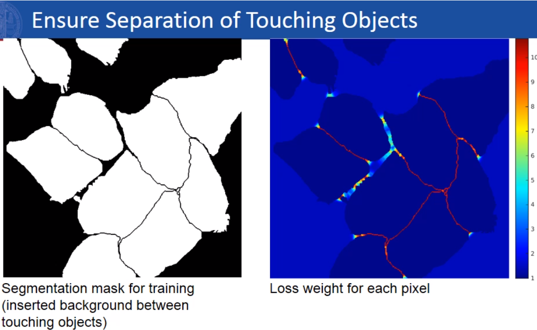
- The use of a weighted loss, where the separating background labels between touching cells of the same class
- Overlap-tile strategy for seamless segmentation of arbitrary large images
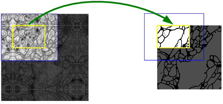
Important trick: select the input tile size such that all 2x2 max-pooling operations are applied to a layer with an even x- and y-size
- shift
- rotation
- random elastic deformations:
smooth deformations using random displacement vectors on a coarse 3 by 3 grid.
The displacements are sampled from a Gaussian distribution with 10 pixels standard deviation.
Per-pixel displacements are then computed using bicubic interpolation.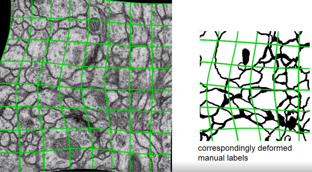
- Drop-out
Challenge in medical image
: The anatomy of interest occupies only a very small region of the scan, which causes the learning process to get trapped in local minima of loss function yielding a network whose predictions are strongly biased towards background.
As a result the foreground region is often missing or only partially detected.
-
CrossEntropyLoss (Naive Method) Works badly for two reasons:
1)highly unbalanced label distribution
2)per-pixel intrinsic issue of cross entropy loss
As a result, cross entropy loss only considers loss in a micro sense rather than considering it globally, which is not enoujgh for image level prediction. -
Dice Loss Originates from Sørensen–Dice coefficient, which is a statistic developed in 1940s to gauge the similarity between two samples.It was brought to computer vision community by Milletari et al.in 2016 for 3D medical image segmentation.
Below shows the equation of Dice coefficient, in which p and q represent pairs of corresponding pixel values of prediction and ground truth, respectively. Its quantity range between 0 and 1 which we aim to maximize.

Dice loss considers the loss information both locally and globally, which is critical for high accuracy.
If you are interested in segmentation loss functions much in depth, you will find this repository helpful : https://github.com/JunMa11/SegLoss