This repository provides an example of PYNQ supporting multiple boards from a single pip-installable package. From the same HLS/SDSoC source code, and using the same Python API and notebooks, we can develop applications which simply move across Xilinx boards. This has the potential to simplify the deployment of code in embedded applications, improve reusability and reduce design time.
Open a terminal on your PYNQ board and run:
sudo pip3 install --upgrade git+https://github.com/sfox14/pynq-ekf.git
This will install the pynq-ekf package to your board, and will create the ekf directory in the PYNQ_JUPYTER_NOTEBOOKS path. Here you will find notebooks which test our EKF design.
gps_notebook.ipynb- the application of EKF in gpslight_notebook.ipynb- a sensor fusion example using KF and board I/O
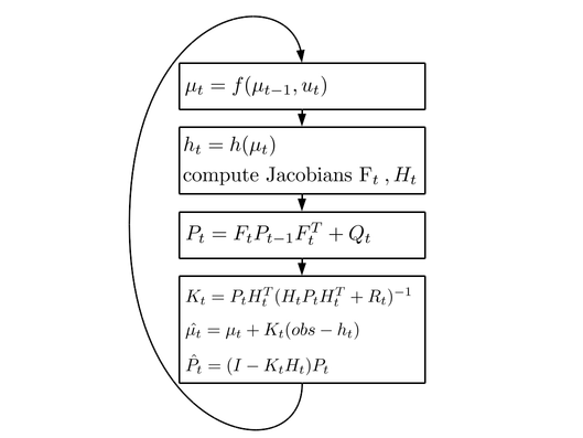
The Kalman Filter (KF) and Extended Kalman Filter (EKF) are recursive state estimators for linear and non-linear systems respectively, with additive white noise. KFs are optimal estimators whereas EKFs have to make an approximation. This is because linear functions of Gaussian variables are themselves Gaussian, and hence the posterior probability distribution function (PDF) can be computed exactly, applying matrix operators without doing any sampling. This also has computational benefits since the majority of modern processors are good at handling matrices. To leverage the benefits of linear models, for non-linear signals, EKFs find an approximation by linearising around an estimate of the non-linear function's mean. Linearisation is the same as computing the gradient, which means that matrices of partial derivatives (i.e. Jacobian matrices) need to be computed for each iteration or state estimate. Kalman Filtering is a prediction technique for modelling uncertainty, and therefore every variable and function has an associated mean and covariance which is assumed Gaussian. KFs and EKFs work by combining two noisy models, a process or state transition function (f) and observation function (h), and trade off the uncertainties of each to form a better estimate of the underlying state. This is captured in the computational graph for the EKF below:
For more information on Kalman Filters, this course provides good explanation and notes .
There are two accelerator architectures.
-
Hardware-Software (HW-SW): This design offers flexibility and generality because only the application-independent part of the algorithm is accelerated on the FPGA. The application specific code can be written in software.
-
Hardware-Only (HW): This design can offer higher performance by deploying the entire algorithm on the FPGA.
The size of both architectures is largely determined by two parameters:
- N - the number of states
- M - the number of observations
This repository contains bitstreams and libraries for both architectures, and includes a build flow for rebuilding different (N,M) configurations for the hybrid HW-SW architecture only. In boards\$(BOARD_NAME)\hw-sw, you will see bitstream (and accompanying tcl) files named with an n${N}m${M} suffix to indicate it's configuration. Models/Applications which have the same configuration, can share the same bitstream.
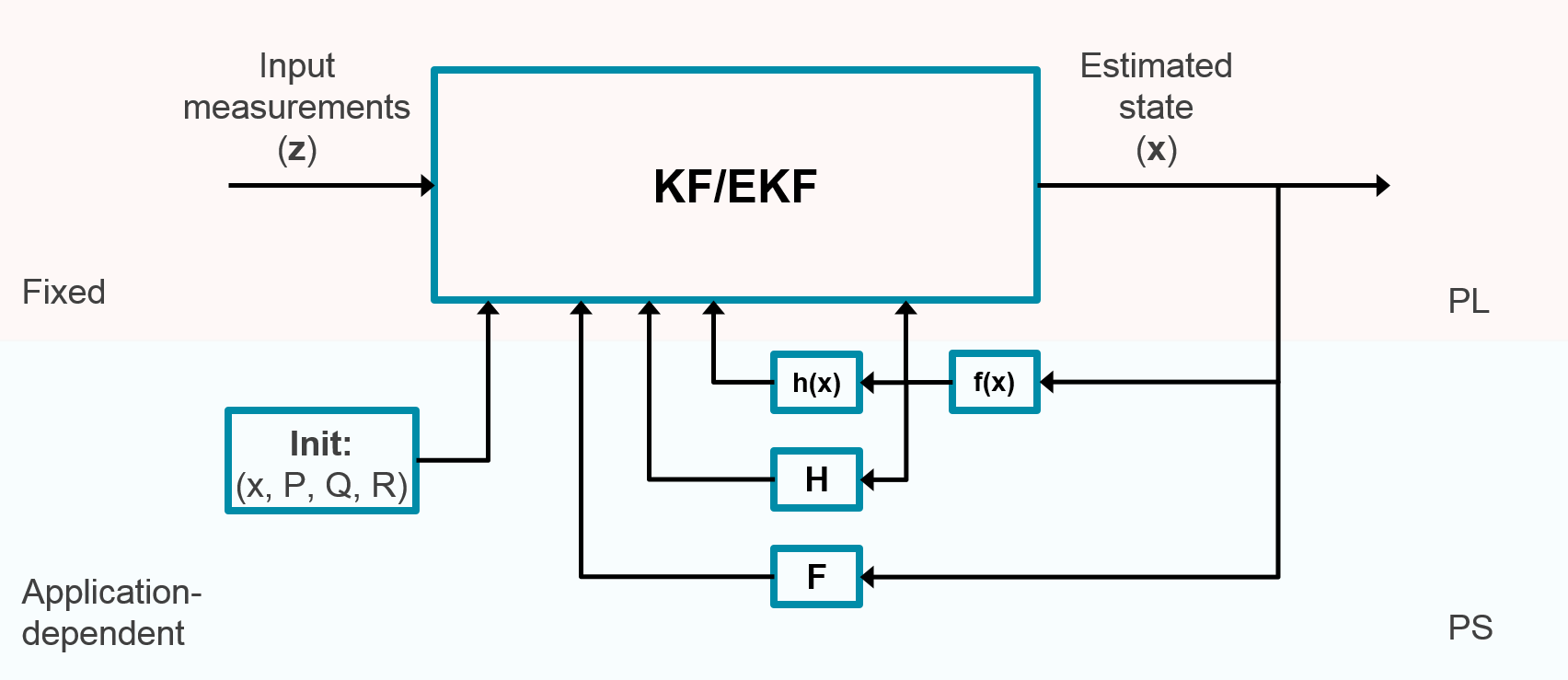
The figure below shows how the computation is separated between Processing System (PS) and Programmable Logic (PL). This design offers runtime flexibility and can be generalised for KF and EKF problems. The state (x) as well as the state covariance (P), process covariance (Q) and observation covariance (R) matrices can be loaded at runtime. Furthermore, the state transition function, f(x), and observation model, h(x), are computed in software on the ARM processor. This allows compatability with more complex systems.
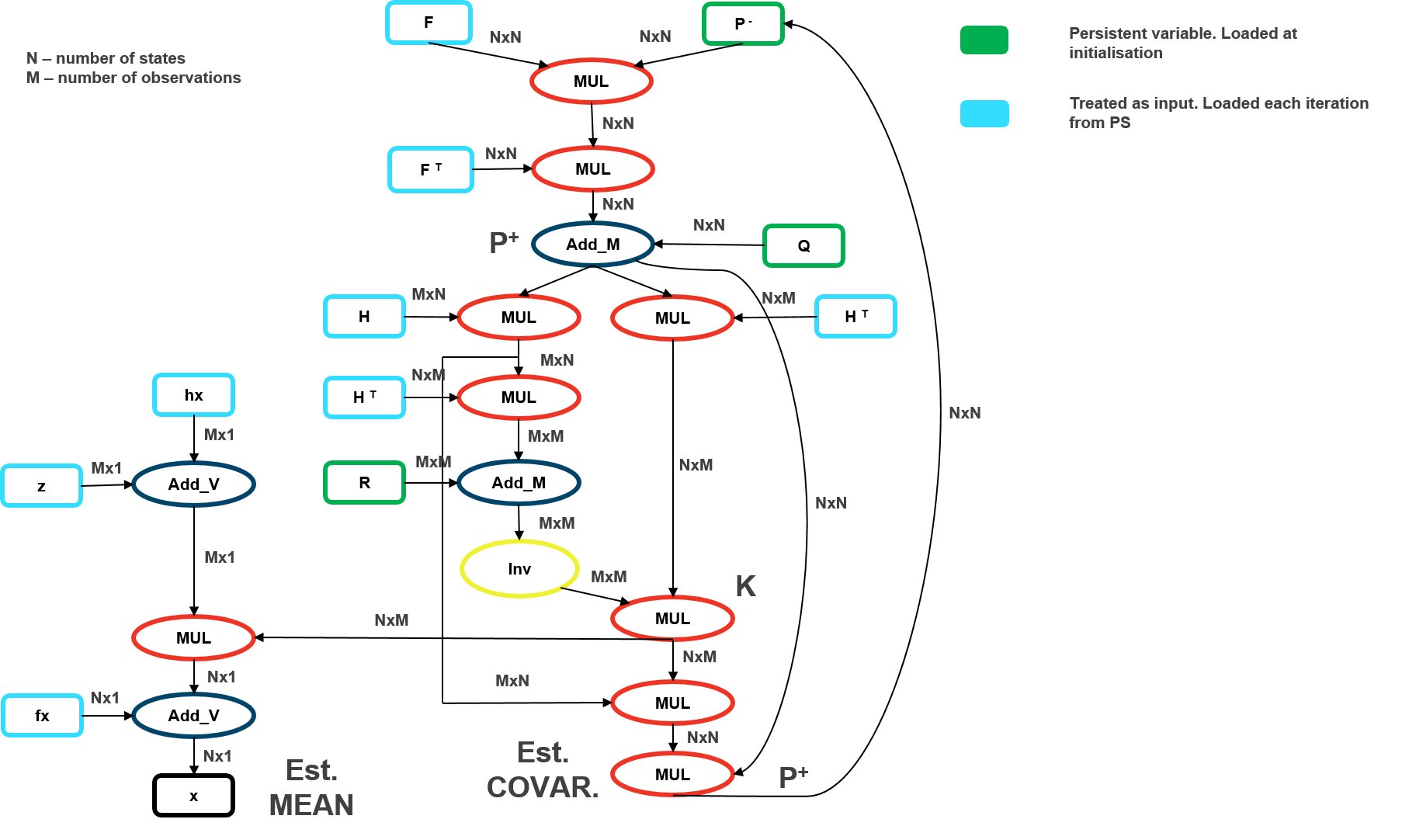
The PL implements the required matrix operations in a dataflow architecture. The figure below gives an illustration of the type and sequence of computation that is performed. The primary computational bottleneck is the matrix inversion. We implemented this via LU Decomposition (app note). This design requires a relatively large amount of data from external memory each iteration. On small problems, this approach gives bad performance since the majority of time is spent transferring data between processor and FPGA. Furthermore, converting between Fixed and Floating point number representations is expensive and further reduces system throughput/performance.
Given the performance drawbacks of the HW-SW co-design, it may be better to implement the entire algorithm on the FPGA. The gps_example.ipynb notebook gives an example for this, however this option can not support other EKF applications or configurations.
The following table shows an example performance (execution time in milliseconds) of the EKF accelerator for the GPS example. It assumes a model with N=8 states and M=4 observations, and is the same as the C/C++ model implemented here. The dataset is generated in make_dataset.py, and characterises a typical GPS system. The execution time was measured for SW-only, HW-only and hybrid HW-SW designs.
| Board | PL Clock /MHz |
TinyEKF (C) |
Naive SW (Python) |
HW-SW (Python) |
HW-only (Python) |
|---|---|---|---|---|---|
| Pynq-Z1 | 100 | 15.2 | 64.1 | 83.3 | 1.8 |
| ZCU104 | 250 | 9.5 | 27.7 | 37.1 | 0.7 |
Note that Zynq Ultrascale boards such as ZCU104 in general have more cores, higher CPU frequency, higher PL clock rates, and larger DDR memory size.
Follow the instructions to rebuild the EKF. This repository contains prebuilt bitstreams and libraries for SDSoC projects built against Pynq-Z1, Ultra96 and ZCU104 boards. You must have a valid Xilinx license for Vivado and SDSoC 2017.4 to run the makefile.
boards: List of boards currently supported, with their associated bitstreams and libraries.Pynq-Z1/Pynq-Z2/Ultra96/ZCU104/etc: Supported boardsgps/n2m2/etc: various designs with their bitstreams and metadata.notebooks: notebooks copied into the jupyter notebook location.
build: The source and scripts to rebuild the projectssrc: HLS/SDSoC source files
ekf: Python source and API. Each design inherits from a base class and implements their own model.ekf.py: contains the EKF base classgps_ekf.py: python class for the GPS examplelight_ekf.py: python class for the Light sensor-fusion example
utils: Extra repository stuffimages: Pictures, illustrations and tablespython: Code for generatinggps_data.csvandparams.dattiny-ekf: An adapted version of TinyEKF for our generated GPS dataset. Used to benchmark performance.
-
Kalman Filter Notes and Slides - Online lectures and notes given on EKF by Cyril Stachniss (Albert-Ludwigs-Universität Freiburg).
-
TinyEKF - An example C/C++ and Python implementation of EKF for Arduino. This repository also contains working C code for the gps example.
PYNQ License : BSD 3-Clause License
TinyEKF License : MIT License


