Shiming Zhou
Using devices such as Jawbone Up, Nike FuelBand, and Fitbit it is now possible to collect a large amount of data about personal activity relatively inexpensively. These type of devices are part of the quantified self movement, One thing that people regularly do is quantify how much of a particular activity they do, but they rarely quantify how well they do it. In this project, we use data from accelerometers on the belt, forearm, arm, and dumbell of 6 participants. They were asked to perform barbell lifts correctly and incorrectly in 5 different ways. And the result can potentially provide useful information for a large variety of applications,such as sports training.
- We use dataset which include records from accelerometers on belt, foreare, arm and dumbell of 6 participants who perform barbell lifts in 5 different ways (include correct and incorrect ways) to build our predictive models.
- Make feature plots to explore unrelated variabls and exclude them from dataset. And exclude variables including missing values because NA account for 98% observations in those variable including missing values.
- Data spliting: 70% - training data; 30% - test data, to validate the model.
- Built 4 predictive models using different algorithms. Including RandomForest and Generalized Boosting. Each were build w/ and w/o Principle Component Analysis.
- Used 3-fold cross validation to train the Boosting models. No CV for RandomForest, since OOB (out of bag) estimation of out-of-sample error asymptotically equivalent to LOOCV as the number of trees increases (here 500)
- Used test data to built Confusion Matrix and get the accuracy for each model.
- Plot the relationship between Processing Time and Accuracy for each model. And made heatmaps of Condusion Matrix for RandomForest and Boosting with PCA models.
- Chose RandomForest as the final model (more than 99% accuracy, around 5 minutes processing time) and make prediction of the 20 test cases.
- Rank the variable importance based on MeanDecreasGini.
The introduction of the WLE dataset Qualitative Activity Recognition of Weight Lifting Exercises Six young health participants were asked to perform one set of 10 repetitions of the Unilateral Dumbbell Biceps Curl in five different fashions: exactly according to the specification (Class A), throwing the elbows to the front (Class B), lifting the dumbbell only halfway (Class C), lowering the dumbbell only halfway (Class D) and throwing the hips to the front (Class E).
Class A corresponds to the specified execution of the exercise, while the other 4 classes correspond to common mistakes. Participants were supervised by an experienced weight lifter to make sure the execution complied to the manner they were supposed to simulate. The exercises were performed by six male participants aged between 20-28 years, with little weight lifting experience. We made sure that all participants could easily simulate the mistakes in a safe and controlled manner by using a relatively light dumbbell (1.25kg).
Data are collected using an on-body sensing approach and "ambient sensing approach".
Training dataset: 19622 observations and 160 variables.
We are going to predict the exercise class for the testing data which include 20 observations.
More information is available from the website here: Human Activity Recognition (see the section on the Weight Lifting Exercise Dataset).
library(downloader)
download("https://d396qusza40orc.cloudfront.net/predmachlearn/pml-training.csv", destfile="training.csv")
download("https://d396qusza40orc.cloudfront.net/predmachlearn/pml-testing.csv", destfile="testing.csv")library(AppliedPredictiveModeling)
library(ggplot2)
training <- read.csv("training.csv", na.string="#DIV/0!")
testing <- read.csv("testing.csv", na.string="#DIV/0!")library(caret)
names(training)[1:7]## [1] "X" "user_name" "raw_timestamp_part_1"
## [4] "raw_timestamp_part_2" "cvtd_timestamp" "new_window"
## [7] "num_window"
featurePlot(x=training[,1:7], y=training$classe, plot="pairs")
training <- training[,-c(1:7)]
testing <- testing[,-c(1:7)]
From the pair plots, We can see that the first seven variables make no sence to the classe prediction, the first column is the seriel number of the observations. and the prediction should not consider the participants's name, the activity time, etc when building the model used for make generalized prediction in the future. Therefore, we removed the first seven variables from the dataset.
##  max_roll_belt   max_picth_belt  min_roll_belt   min_pitch_belt
##  NA     :19216   NA     :19216   NA     :19216   NA     :19216
##  -87.9  :   11   18     :  100   -87.8  :   12   17     :  114
##  166    :   11   5      :   65   -88.2  :   12   2      :   52
##  -87.6  :   10   3      :   50   -87.7  :   10   3      :   50
##  -87.7  :   10   4      :   40   161    :   10   4      :   50
##  -88.2  :   10   20     :   36   -88.4  :    9   18     :   45
##  (Other):  354   (Other):  115   (Other):  353   (Other):   95
##  amplitude_roll_belt amplitude_pitch_belt var_total_accel_belt
##  NA     :19216       NA     :19216        NA     :19216
##  0.2    :   40       1      :  216        0.2    :  117
##  1      :   31       2      :   71        0.1    :   82
##  0.3    :   27       0      :   32        0      :   59
##  0.1    :   26       3      :   18        0.3    :   52
##  0.4    :   18       4      :   13        0.4    :    8
##  (Other):  264       (Other):   56        (Other):   88
##  avg_roll_belt   stddev_roll_belt var_roll_belt   avg_pitch_belt
##  NA     :19216   NA     :19216    NA     :19216   NA     :19216
##  1.3    :   16   0.1    :   53    0      :  126   4.5    :   11
##  1.1    :   15   0.4    :   51    0.1    :   78   -43.6  :    8
##  1.5    :   15   0.5    :   50    0.2    :   56   4.6    :    8
##  0.7    :   14   0.2    :   46    0.3    :   23   5      :    8
##  0.8    :   14   0.3    :   41    0.4    :   10   25.5   :    7
##  (Other):  332   (Other):  165    (Other):  113   (Other):  364
##  stddev_pitch_belt var_pitch_belt   avg_yaw_belt   stddev_yaw_belt
##  NA     :19216     NA     :19216   NA     :19216   NA     :19216
##  0.2    :   72     0      :  119   -88    :   12   0.1    :   83
##  0.3    :   62     0.1    :   91   -87.9  :   10   0.2    :   49
##  0.1    :   57     0.2    :   38   -88.2  :   10   0      :   44
##  0.4    :   38     0.3    :   22   -87.7  :    9   0.5    :   35
##  0.5    :   24     0.4    :   14   -87.8  :    7   0.4    :   32
##  (Other):  153     (Other):  122   (Other):  358   (Other):  163
##   var_yaw_belt   var_accel_arm     avg_roll_arm   stddev_roll_arm
##  NA     :19216   NA     :19216   NA      :19216   NA     :19216
##  0      :   66   0      :   11   0       :   77   0      :   77
##  0.01   :   44   0.1582 :    2   -0.7853 :    1   0.05   :    1
##  0.02   :   24   0.0179 :    1   -1.9176 :    1   0.1081 :    1
##  0.03   :   16   0.02   :    1   -10.8644:    1   0.2323 :    1
##  0.25   :   13   0.0222 :    1   -10.9094:    1   0.3331 :    1
##  (Other):  243   (Other):  390   (Other) :  325   (Other):  325
##   var_roll_arm   avg_pitch_arm   stddev_pitch_arm var_pitch_arm
##  NA     :19216   NA     :19216   NA     :19216    NA     :19216
##  0      :   77   0      :   77   0      :   77    0      :   77
##  0.0025 :    1   -0.3724:    1   0.0153 :    1    0.0182 :    1
##  0.0117 :    1   -0.4137:    1   0.135  :    1    0.0275 :    1
##  0.054  :    1   -0.5892:    1   0.1657 :    1    0.0488 :    1
##  0.111  :    1   -0.6586:    1   0.2209 :    1    0.067  :    1
##  (Other):  325   (Other):  325   (Other):  325    (Other):  325
##    avg_yaw_arm    stddev_yaw_arm   var_yaw_arm     max_roll_arm
##  NA      :19216   NA     :19216   NA     :19216   NA     :19216
##  0       :   77   0      :   80   0      :   80   0      :   77
##  -0.0188 :    1   0.3471 :    1   0.1205 :    1   16.8   :    3
##  -0.07   :    1   0.3594 :    1   0.1292 :    1   20.4   :    3
##  -10.4154:    1   0.4552 :    1   0.2072 :    1   30.5   :    3
##  -10.8806:    1   0.4871 :    1   0.2373 :    1   8.5    :    3
##  (Other) :  325   (Other):  322   (Other):  322   (Other):  317
##  max_picth_arm    max_yaw_arm     min_roll_arm   min_pitch_arm
##  NA     :19216   NA     :19216   NA     :19216   NA     :19216
##  0      :   77   32     :   27   0      :   77   0      :   77
##  108    :    6   33     :   22   -41.9  :    4   -113   :    4
##  113    :    5   30     :   19   -23.1  :    3   -103   :    3
##  102    :    4   34     :   19   -37.1  :    3   -104   :    3
##  103    :    4   31     :   18   -43.5  :    3   -108   :    3
##  (Other):  310   (Other):  301   (Other):  316   (Other):  316
##   min_yaw_arm    amplitude_roll_arm amplitude_pitch_arm amplitude_yaw_arm
##  NA     :19216   NA     :19216      NA     :19216       NA     :19216
##  10     :   26   0      :   77      0      :   80       1      :   28
##  5      :   26   1.3    :    3      1      :    4       22     :   27
##  13     :   25   15.7   :    3      125.2  :    3       21     :   18
##  14     :   22   1.6    :    2      132.8  :    3       24     :   17
##  7      :   21   17.9   :    2      2      :    3       25     :   17
##  (Other):  286   (Other):  319      (Other):  313       (Other):  299
##  max_roll_dumbbell max_picth_dumbbell min_roll_dumbbell min_pitch_dumbbell
##  NA     :19216     NA     :19216      NA     :19216     NA     :19216
##  -36.4  :    4     14.7   :    4      -59    :    4     0      :    5
##  -38.2  :    4     -38.2  :    3      0      :    4     -22.4  :    3
##  -49.4  :    4     101.2  :    3      -32.7  :    3     -38.2  :    3
##  -49.7  :    3     126.4  :    3      -33.1  :    3     -81.6  :    3
##  16.8   :    3     134.9  :    3      -38    :    3     -85.8  :    3
##  (Other):  388     (Other):  390      (Other):  389     (Other):  389
##  amplitude_roll_dumbbell amplitude_pitch_dumbbell var_accel_dumbbell
##  NA     :19216           NA     :19216            NA     :19216
##  0      :   16           0      :   16            0      :   18
##  19.31  :    2           118.4  :    2            0.1949 :    3
##  2.72   :    2           13.45  :    2            0.0217 :    2
##  20.11  :    2           21.76  :    2            0.4311 :    2
##  29.48  :    2           23.88  :    2            1.3929 :    2
##  (Other):  382           (Other):  382            (Other):  379
##  avg_roll_dumbbell stddev_roll_dumbbell var_roll_dumbbell
##  NA       :19216   NA     :19216        NA     :19216
##  -101.5169:    3   0      :   16        0      :   16
##  125.9932 :    3   0.1811 :    1        0.0328 :    1
##  52.66    :    3   0.2994 :    1        0.0896 :    1
##  -107.4901:    2   0.3015 :    1        0.0909 :    1
##  109.2254 :    2   0.3665 :    1        0.1343 :    1
##  (Other)  :  393   (Other):  386        (Other):  386
##  avg_pitch_dumbbell stddev_pitch_dumbbell var_pitch_dumbbell
##  NA      :19216     NA     :19216         NA     :19216
##  -38.2221:    3     0      :   16         0      :   16
##  16.8326 :    3     0.2384 :    1         0.0568 :    1
##  27.1869 :    3     0.246  :    1         0.0605 :    1
##  -43.9609:    2     0.2687 :    1         0.0722 :    1
##  -61.3062:    2     0.2798 :    1         0.0783 :    1
##  (Other) :  393     (Other):  386         (Other):  386
##  avg_yaw_dumbbell stddev_yaw_dumbbell var_yaw_dumbbell max_roll_forearm
##  NA      :19216   NA     :19216       NA     :19216    NA     :19216
##  -38.2221:    3   0      :   16       0      :   16    0      :   83
##  101.2451:    3   0.256  :    1       0.0656 :    1    -63.7  :    3
##  14.7001 :    3   0.2581 :    1       0.0666 :    1    23.7   :    3
##  -22.378 :    2   0.2864 :    1       0.082  :    1    28.8   :    3
##  21.4432 :    2   0.3249 :    1       0.1056 :    1    29.6   :    3
##  (Other) :  393   (Other):  386       (Other):  386    (Other):  311
##  max_picth_forearm min_roll_forearm min_pitch_forearm
##  NA     :19216     NA     :19216    NA     :19216
##  0      :   83     0      :   83    0      :   83
##  179    :   28     -0.4   :    3    -179   :   29
##  178    :   20     -13.8  :    3    -178   :   25
##  176    :   16     -2.7   :    3    -180   :   17
##  177    :   14     12.8   :    3    -176   :   13
##  (Other):  245     (Other):  311    (Other):  239
##  amplitude_roll_forearm amplitude_pitch_forearm var_accel_forearm
##  NA     :19216          NA     :19216           NA     :19216
##  0      :   83          0      :   85           0      :    7
##  1.7    :    4          354    :   26           0.02326:    2
##  0.3    :    3          356    :   13           0.03634:    1
##  1      :    3          358    :   13           0.06082:    1
##  2.7    :    3          1      :   12           0.06753:    1
##  (Other):  310          (Other):  257           (Other):  394
##  avg_roll_forearm stddev_roll_forearm var_roll_forearm avg_pitch_forearm
##  NA      :19216   NA     :19216       NA     :19216    NA      :19216
##  0       :   83   0      :   87       0      :   87    0       :   83
##  148     :    3   0.13736:    1       0.01887:    1    -0.38473:    1
##  -0.04542:    1   0.20927:    1       0.04379:    1    -0.56106:    1
##  -0.71875:    1   0.23772:    1       0.05651:    1    -0.59022:    1
##  -0.97204:    1   0.24204:    1       0.05858:    1    -0.84531:    1
##  (Other) :  317   (Other):  315       (Other):  315    (Other) :  319
##  stddev_pitch_forearm var_pitch_forearm   avg_yaw_forearm
##  NA     :19216        NA     :19216     NA        :19216
##  0      :   83        0      :   83     0         :   83
##  0.82447:    2        0.00043:    1     -1.07213  :    1
##  0.02082:    1        0.00371:    1     -1.5242   :    1
##  0.06088:    1        0.00559:    1     -10.14286 :    1
##  0.07474:    1        0.00611:    1     -100.77442:    1
##  (Other):  318        (Other):  319     (Other)   :  319
##  stddev_yaw_forearm var_yaw_forearm classe
##  NA     :19216      NA     :19216   A:5580
##  0      :   85      0      :   85   B:3797
##  0.06047:    1      0.00366:    1   C:3422
##  0.19024:    1      0.03619:    1   D:3216
##  0.20841:    1      0.04343:    1   E:3607
##  0.21308:    1      0.0454 :    1
##  (Other):  317      (Other):  317
From the summary for factor variables, we found that All the factor variables have 19216 NAs, we can see a pattern for the existed NA valudes, and the NA values acount for 98% observations, We remove all the factor variables.
colNA <- colSums(is.na(trainingNF))
training1 <- trainingNF[, which(colNA==0)]
trainingFinal <- cbind(training1, classe = training$classe)
testing1 <- testingNF[, which(colNA==0)]
testingFinal <- cbind(testing1, classe = testing$problem_id)
all those remaining columns, which include NAs, have more than 19000 NAs, means more than 98% of the values for corresponding columes are missing, indicating that those variables have little influence to the final exercise quality. therefore, we remove them and got our training1 dataframe, after add the classe column from the original dataframe, we got our final data set trainingFinal which include 52 predictors after exclude the classe column.
we use 70% of the training data to train our model, and use the remaining 30% to validate our model
set.seed(123)
useData <- createDataPartition(y=trainingFinal$classe, p=0.7, list=FALSE)
myTraining <- trainingFinal[useData,]
myTesting <- trainingFinal[-useData,]- we may not need every predictor
- PCA is and effective way in reducing the size of the problem without losing much accuracy.
- We set the threshold cumulative variance to 80%.
- Omission of PCA permits variable importance ranking, a nice insight into the problem.
preProc <- preProcess(myTraining[,-53], method="pca", thresh=.8)
myTrainingPC <- predict(preProc, myTraining[,-53])
myTestingPC <- predict(preProc, myTesting[,-53])Use doSNOW for doing parallel processing
library(doSNOW)
registerDoSNOW(makeCluster(2, type = "SOCK"))We select RandomForest and Boosting, the top 2 performing algorithms in predicting contents, to build our model. For each algorithm, we build two models w/ and w/o PCA preprocessing.
- Breiman's random forest algorithm (based on Breiman and Cutler's original Fortran code) for classification.
- Using 500 trees and mtry = square root of p, the number of predictors(equals to 7 in this case)
- Cross Validation: not required for random forests, since each tree uses, on average, 2/3 of the observations, OOB (out of bag) estimation of out-of-sample error is valid and is asymptotically equivalent to LOOCV as the number of trees increases (here 500)
##
## Call:
##  randomForest(formula = myTraining$classe ~ ., data = myTrainingPC,      importance = TRUE, proximity = TRUE)
##                Type of random forest: classification
##                      Number of trees: 500
## No. of variables tried at each split: 3
##
##         OOB estimate of  error rate: 4.24%
## Confusion matrix:
##      A    B    C    D    E class.error
## A 3813   23   40   23    7     0.02381
## B   68 2499   67   11   13     0.05982
## C   21   39 2295   30   11     0.04215
## D   23   11  115 2092   11     0.07105
## E    4   20   20   26 2455     0.02772
##
## Call:
##  randomForest(formula = classe ~ ., data = myTraining, importance = TRUE,      proximity = TRUE)
##                Type of random forest: classification
##                      Number of trees: 500
## No. of variables tried at each split: 7
##
##         OOB estimate of  error rate: 0.57%
## Confusion matrix:
##      A    B    C    D    E class.error
## A 3902    2    0    0    2    0.001024
## B   12 2640    6    0    0    0.006772
## C    0   16 2377    3    0    0.007930
## D    0    0   27 2224    1    0.012433
## E    0    0    3    6 2516    0.003564
- Boosting is the process of iteratively adding basis functions in a greedy fashion so that each additional basis function further reduces the selected loss function.
- We use generalized boosted with trees model
- Using 500 trees and Max Tree Depth = 3, shrinkage = .1,
- Cross Validation: Used for better estimating how accurately a predictive model will perform in practice. Number of cross-validation folds equals to 3, and we will get an estimate of generalization error
## Stochastic Gradient Boosting
##
## 13737 samples
##    52 predictor
##     5 classes: 'A', 'B', 'C', 'D', 'E'
##
## No pre-processing
## Resampling: Cross-Validated (3 fold)
##
## Summary of sample sizes: 9157, 9157, 9160
##
## Resampling results
##
##   Accuracy  Kappa  Accuracy SD  Kappa SD
##   1         1      0.001        0.002
##
## Tuning parameter 'n.trees' was held constant at a value of 500
##
## Tuning parameter 'interaction.depth' was held constant at a value of
##  3
## Tuning parameter 'shrinkage' was held constant at a value of 0.1
##
## Stochastic Gradient Boosting
##
## 13737 samples
##    11 predictor
##     5 classes: 'A', 'B', 'C', 'D', 'E'
##
## No pre-processing
## Resampling: Cross-Validated (3 fold)
##
## Summary of sample sizes: 9157, 9157, 9160
##
## Resampling results
##
##   Accuracy  Kappa  Accuracy SD  Kappa SD
##   0.8       0.8    0.007        0.009
##
## Tuning parameter 'n.trees' was held constant at a value of 500
##
## Tuning parameter 'interaction.depth' was held constant at a value of
##  3
## Tuning parameter 'shrinkage' was held constant at a value of 0.1
##
- Processing Time: During the model building process, we use Sys.time to computing time needed to execution expression.
- Accuracy: The accuracy for each model are acquired through the confusion Matrix. Showing the accuracy when predicting the test data using each model. Which equals to (1- out of sample error).
- The following plot the relationship between the process time and the accuracy for each model.
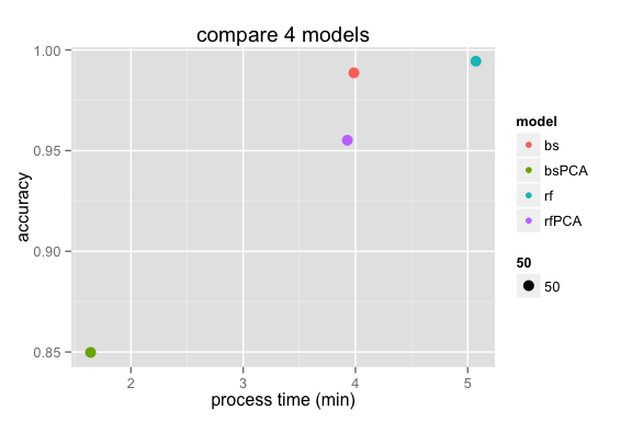

we can see that the randomForest use the longest time but with the highest accuracy. and the boosting with PCA has the lowest accuracy but it only require a little more than 1 minutes.
Now, we want to campare these two models with the heatmaps to show the confusion Matrix, in order to see how these two models predict for each classe.
We normalize the confusion Matrix first and then use the hearmaps to show the normalized frequency.


We can see the rf model can predict for each classe slightly better.
After compare the process time, the accurancy, we choose the randomForest without PCA as our final model to make the prediction of the test cases. Althrough it requires the longest processing time, but 5 minutes are in an acceptable range and we can get a model with really good accuracy(more than 99%).
No PCA required for 99% accuracy. Omission of PCA permits variable importance ranking, which can give a nice insight into the problem.
randomForest (function and pkg, Breiman's algorithm) on a reduced set of predictors using 500 trees and mtry = square root of p (equals to 7 here), the number of predictors.
We use RandomForest Predictive Model (model2) to predict our 20 cases.
##  1  2  3  4  5  6  7  8  9 10 11 12 13 14 15 16 17 18 19 20
##  B  A  B  A  A  E  D  B  A  A  B  C  B  A  E  E  A  B  B  B
## Levels: A B C D E
The following plot shows the variable importance based on the MeanDecreaseGini for each sensor position. And we also gave the variables which has MeanDecreasGini>250.

##                   MeanDecreaseGini AccelPosition    Index
## roll_belt                    879.6          belt     roll
## yaw_belt                     615.0          belt      yaw
## pitch_forearm                536.5       forearm    pitch
## magnet_dumbbell_z            512.1      dumbbell magnet_z
## pitch_belt                   490.2          belt    pitch
## magnet_dumbbell_y            462.4      dumbbell magnet_y
## roll_forearm                 415.2       forearm     roll
## magnet_dumbbell_x            340.1      dumbbell magnet_x
## roll_dumbbell                299.7      dumbbell     roll
## accel_dumbbell_y             286.8      dumbbell  accel_y
## accel_belt_z                 275.4          belt  accel_z
## magnet_belt_z                272.6          belt magnet_z
## magnet_belt_y                263.9          belt magnet_y
From the plot, we can see than the roll_belt and yaw_belt are the most two important variables for the Weight Lifting performance quality. And the varaibles related with arm has least influence to the performance quality.
These results can potentially provide useful information for a large variety of applications,such as sports training. We can get to know which position or what kind of mistake of the exercise caused. These results can also be applied when developing new monitoring advices which focus on helping people to correct their exercises quality.