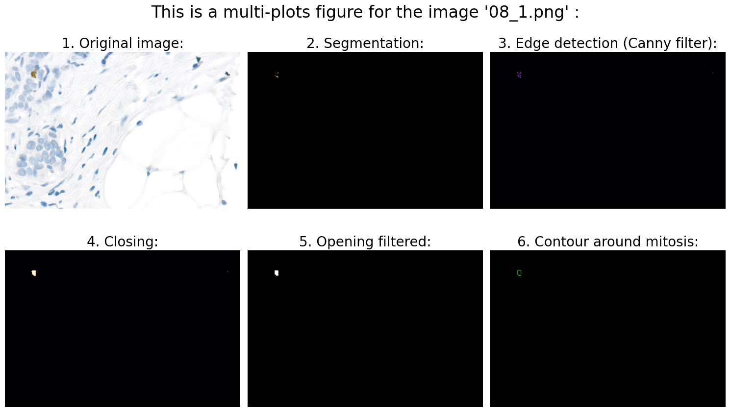
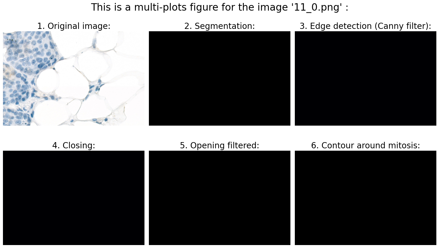
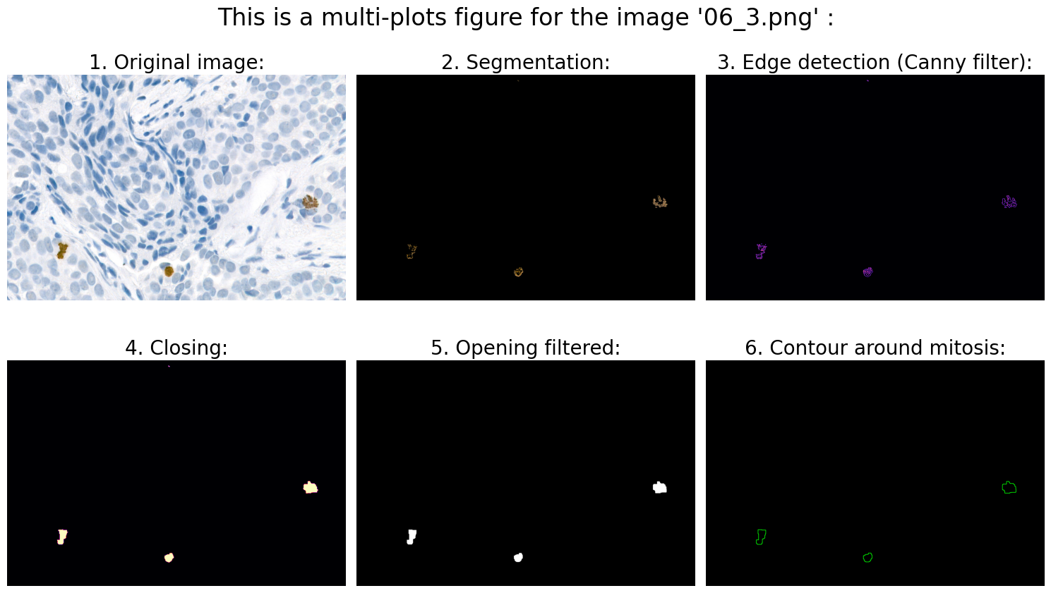
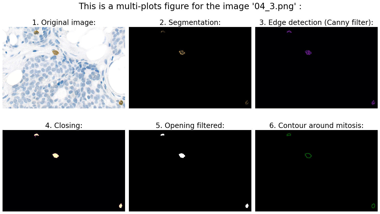
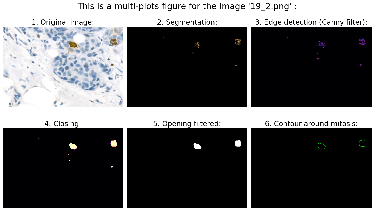
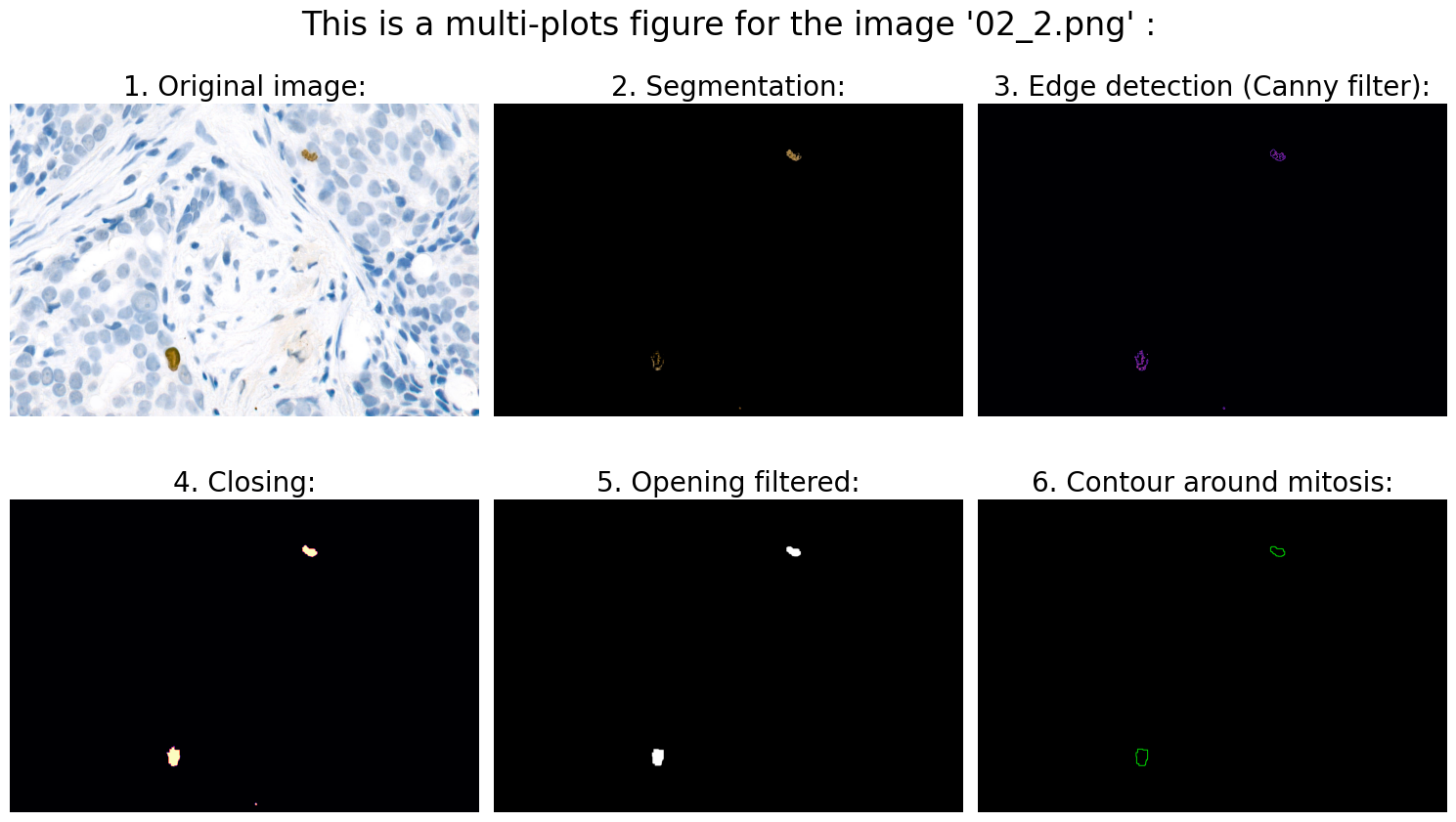
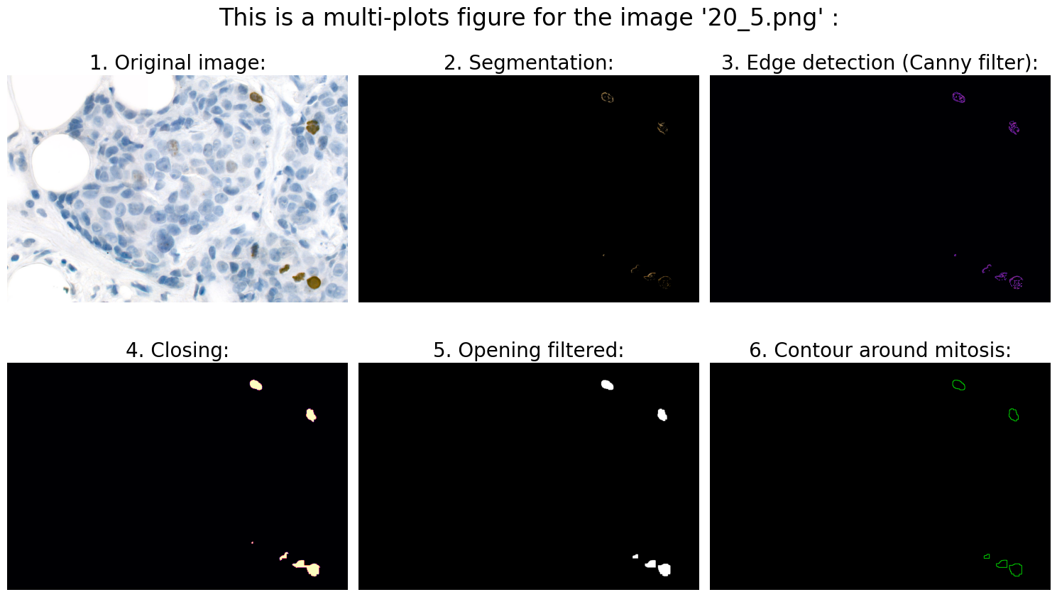
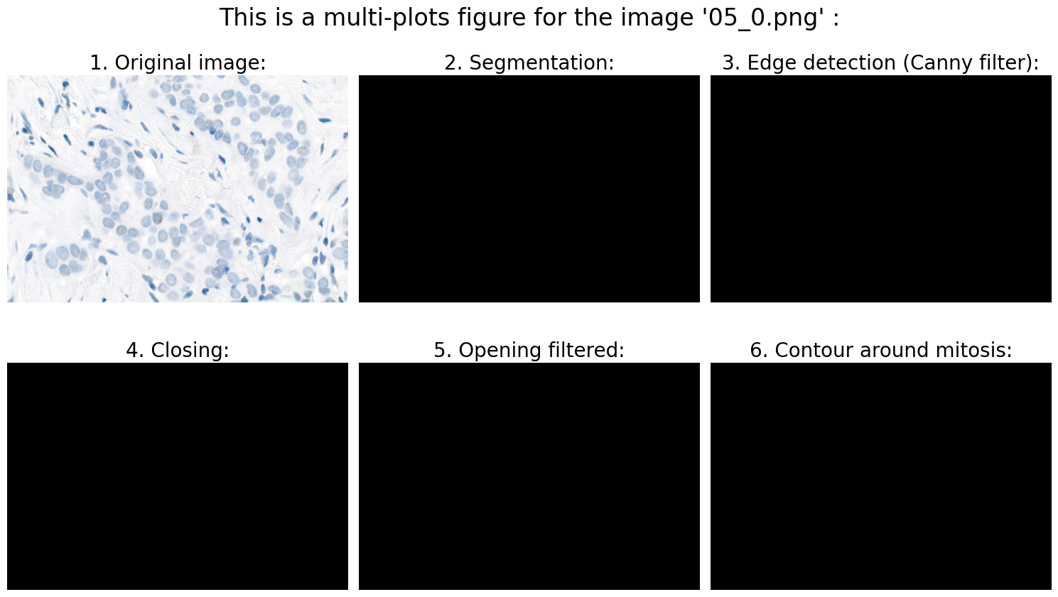
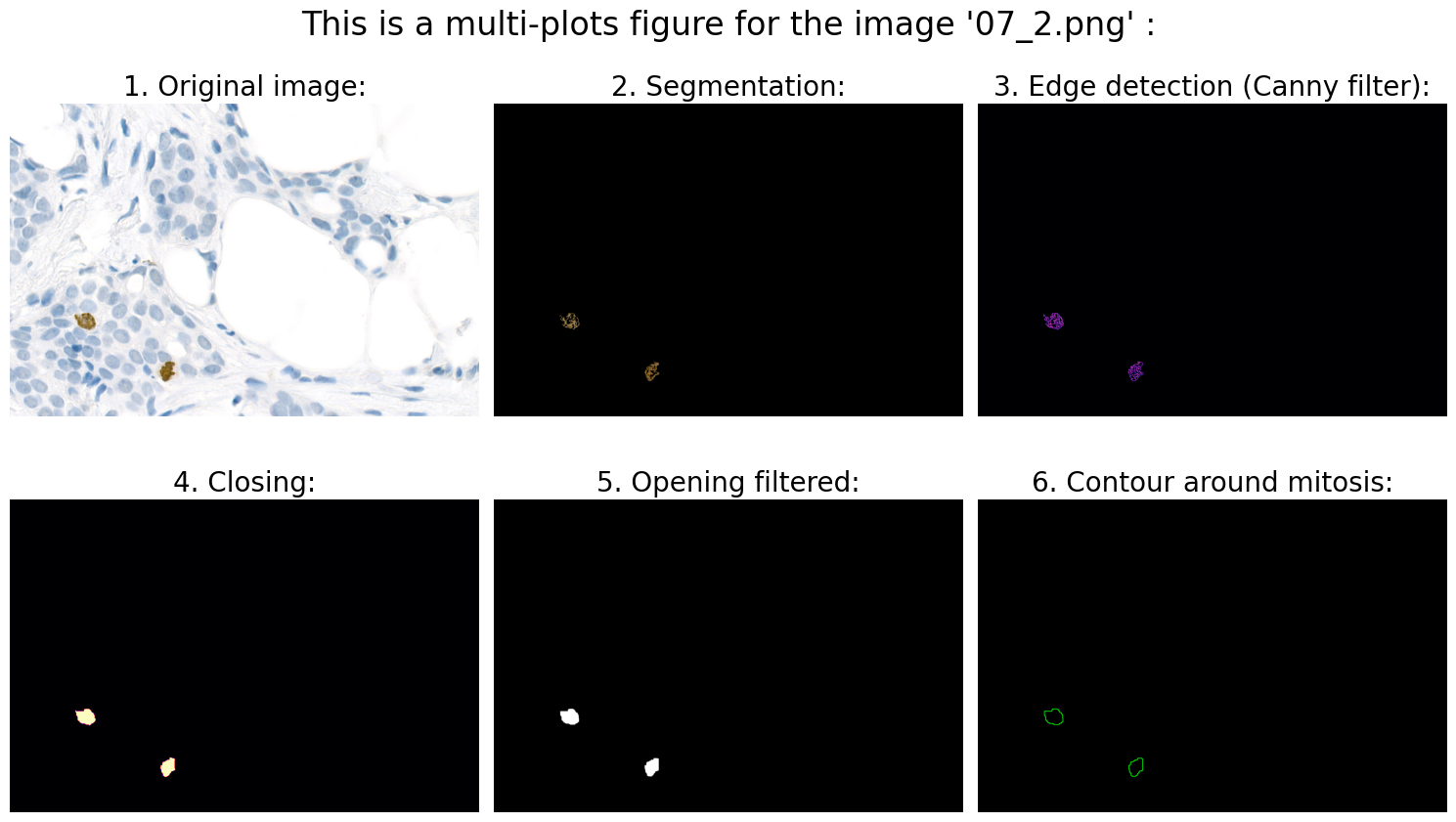
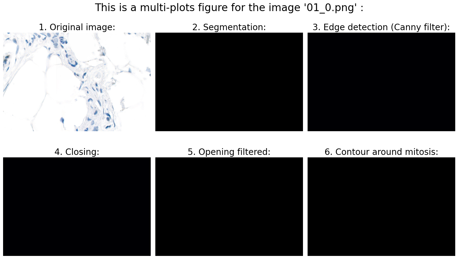
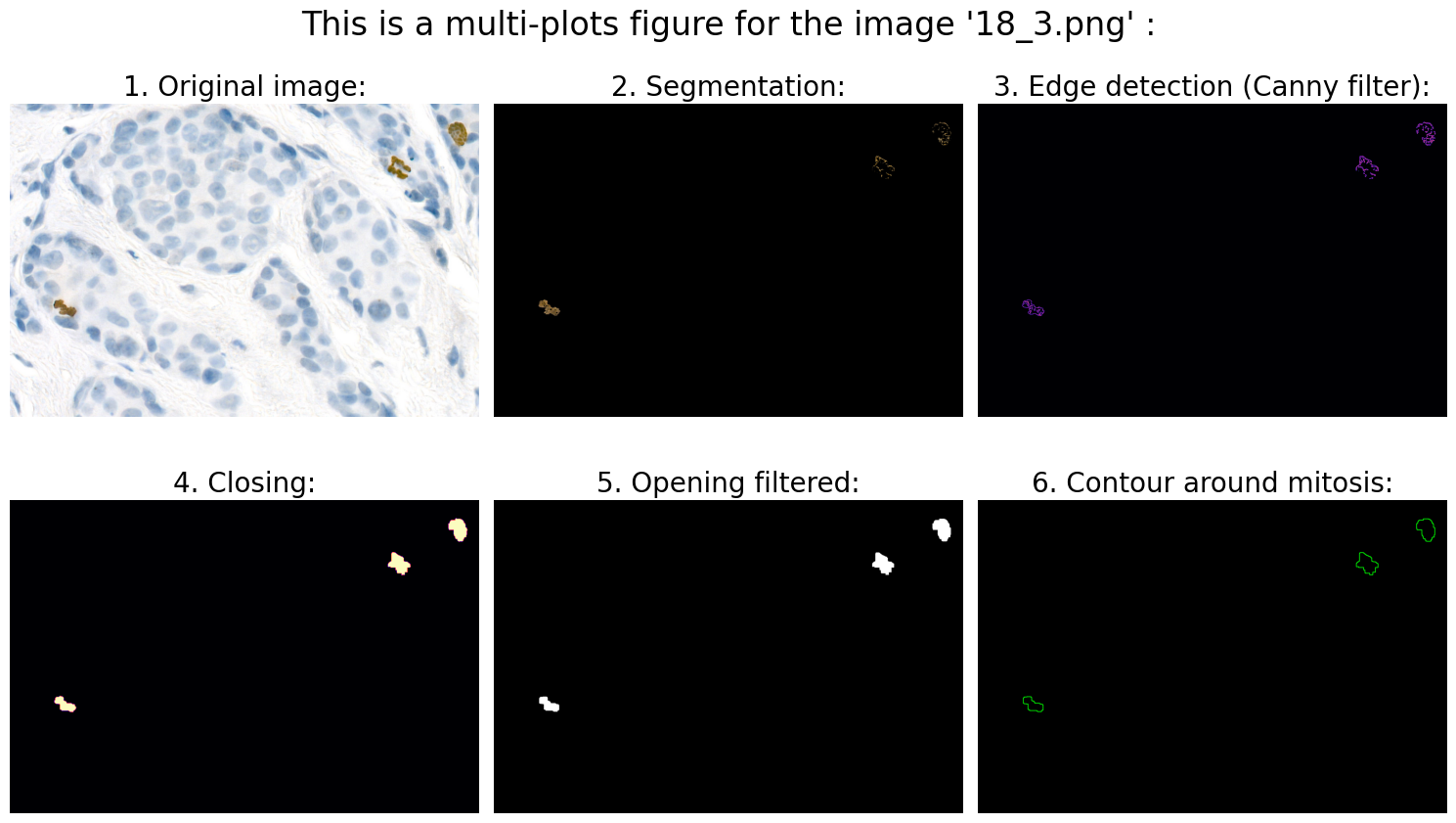
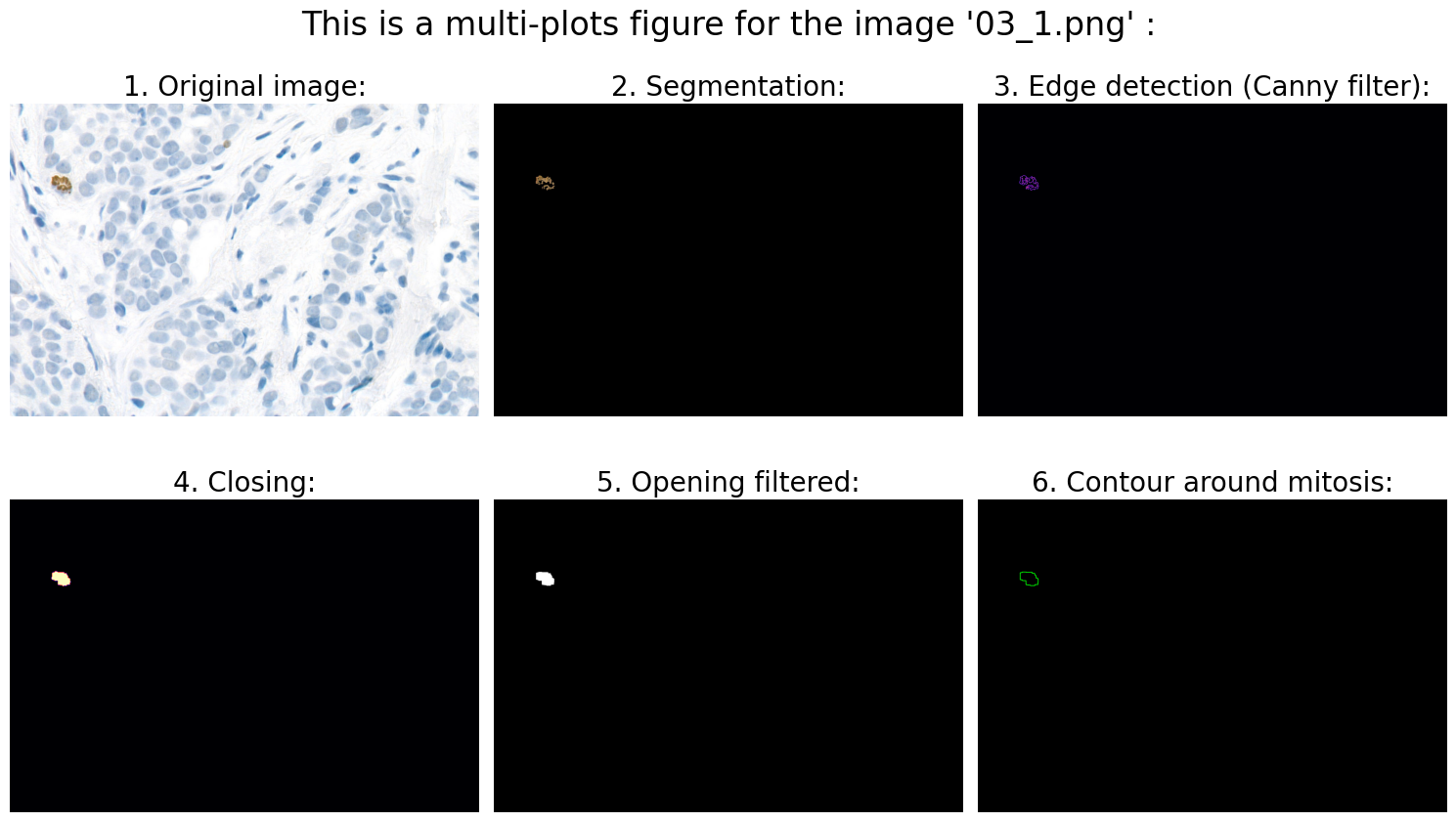
Automated Mitosis Detection and Analysis in Histological Images Using OpenCV and Image Processing Techniques
To run this program, you need to have the following installed:
- Python 3.9 or later
- Miniconda or Anaconda
Follow these steps to set up your environment and install the necessary packages.
Download and install Miniconda for your platform from the official Miniconda website.
Open your terminal and create a new Conda environment with Python 3.9:
conda create --name mitosis_env python=3.9
conda activate mitosis_env
Install the required packages using conda and pip:
conda install numpy matplotlib
pip install imutils opencv-python
To use the Conda environment in Jupyter Notebook, install ipykernel and add the environment:
conda install ipykernel
python -m ipykernel install --user --name=mitosis_env --display-name "Python (mitosis_env)"
Start Jupyter Notebook:
jupyter notebook
- Place your images in the
mitosis_data_set/directory. - Run the Jupyter Notebook and execute the cells to process the images and display the results.
# Plots are displayed inline in the notebook
%matplotlib inline
import numpy as np
import imutils
import argparse
import cv2
import matplotlib.pyplot as plt
from os import listdir
from os.path import isfile, join
# This program finds all mitoses in all 20 photos with 100% accuracy. Please press "p" to check:
answer = input("'Enter' - display only the results, \n'p' - display the results along with an automatic check:\n")
path = "mitosis_data_set/"
files = [f for f in listdir(path) if isfile(join(path, f))]
correct_solutions = 0 # <- for auto-check
for file in files:
# 1.0 Open image:
file_name = file
img = cv2.imread(path + file_name)
# 2.0 Preprocessing:
rgb_img = cv2.cvtColor(img, cv2.COLOR_BGR2RGB) # for demonstration in plot
hsv_img = cv2.cvtColor(rgb_img, cv2.COLOR_RGB2HSV) # for further segmentation
# 3.0 Segmentation:
# 3.1 Define the color range to detect for brown:
lower_brown = np.array([10, 100, 20])
upper_brown = np.array([20, 255, 200])
# Why these values? It is known that mitoses in these images are recognizable as brownish structures.
# Therefore, the HSV range for BROWN color in openCV is needed here:
# https://stackoverflow.com/questions/46112326/what-is-the-range-of-hsv-values-for-brown-color-in-opencv
# By applying a mask for brown, we select all brown objects in the image:
mask_brown = cv2.inRange(hsv_img, lower_brown, upper_brown)
# 3.2 Apply the mask:
result = cv2.bitwise_and(rgb_img, rgb_img, mask=mask_brown)
# 4.0 Object detection:
# 4.1 The goal of this step is to detect geometric objects in a grayscale image after segmentation:
gray = cv2.cvtColor(result, cv2.COLOR_RGB2GRAY)
# 4.2 Algorithm for detecting geometric structures: edge detection -> Canny filter
# (https://www.uni-ulm.de/fileadmin/website_uni_ulm/mawi.inst.070/funken/bachelorarbeiten/bachelorarbeitBekeJungeEnd.pdf)
edges = cv2.Canny(gray, 100, 250) # The second and third arguments are our minVal and maxVal.
# Why these values?
# a) All edges with an intensity greater than "maxVal" are the sure edges.
# b) All edges with an intensity less than "minVal" are definitely not edges.
# c) The edges between the "maxVal" and "minVal" thresholds are classified as edges only if they are connected to a sure edge, otherwise, they are discarded.
# This ratio is a recommendation from Canny! -> https://docs.opencv.org/3.4/da/d5c/tutorial_canny_detector.html
# So, Canny recommended an upper:lower ratio between 2:1 and 3:1. Hence, the most average value 2.5:1 was chosen
# 4.3 Calculation of suitable features:
# First, we need to perform some morphological transformations (closing & opening).
# We want to close gaps within the edges to make the objects more cohesive
# and facilitate the finding of contours:
kernel = np.ones((5, 5), np.uint8)
closing = cv2.morphologyEx(edges, cv2.MORPH_CLOSE, kernel, iterations=7)
# Then we want to remove some noise:
opening = cv2.morphologyEx(closing, cv2.MORPH_OPEN, kernel, iterations=3)
# Why these values? A 5x5 kernel, 7 closing iterations, and 3 opening iterations allow us
# to detect contours of at least 168.5 pixels in size. This is the size
# of the contour found in image '19_2.png' that is not mitosis.
# This means that this configuration is empirically (95% accuracy) quite accurate and sensitive.
# Why?
# Given the image resolution, the nucleus of mammalian cells takes up approximately 41 to 123 pixels.
# Thus, the program is able to recognize contours with an area close to the nucleus of mammalian cells
# at the given image resolution.
# In the next step, we need to eliminate all contours that have too little surface area (<480 pixels, empirically).
# We can now use .findContours and .drawContours
# to retrieve the external contours found by the Canny detection and modified by us ...:
contours, hierarchy = cv2.findContours(opening, cv2.RETR_TREE, cv2.CHAIN_APPROX_SIMPLE)
# Create an empty mask:
mask = np.zeros(opening.shape[:2], dtype=opening.dtype)
# Draw all contours larger than 480 on the mask (see above):
for c in contours:
if cv2.contourArea(c) > 480: # (see above)
x, y, w, h = cv2.boundingRect(c)
cv2.drawContours(mask, [c], 0, (255), -1)
# Apply the mask to the original image:
opening_filtered = cv2.bitwise_and(opening, opening, mask=mask)
# Use .findContours again:
contours_filtered, hierarchy_filtered = cv2.findContours(opening_filtered, cv2.RETR_TREE, cv2.CHAIN_APPROX_SIMPLE)
# ... and draw contour around mitosis on a black background for clarification:
ret, black = cv2.threshold(rgb_img, 255, 255, cv2.THRESH_BINARY)
img_contours = cv2.drawContours(black, contours_filtered, -1, (0, 255, 0), 2)
# 5.0 Analysis:
number_of_objects_in_image = len(contours_filtered)
if answer == "p":
# ---- info + auto-check: ----
file_name_last_char_int = int(file_name[-5])
if number_of_objects_in_image == file_name_last_char_int:
print("Found mitoses in the image " + "'" + file_name + "'" + ":", str(number_of_objects_in_image), "✅")
correct_solutions += 1
else:
print("Found mitoses in the image " + "'" + file_name + "'" + ":", str(number_of_objects_in_image), "❌")
else:
# ------ only info: ------
print("Found mitoses in the image " + "'" + file_name + "'" + ":", str(number_of_objects_in_image))
# 6.0 Visualization:
# 6.1 Define fig:
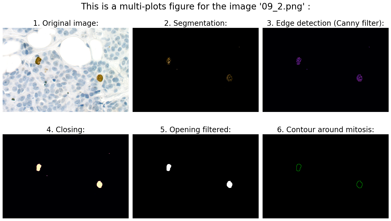
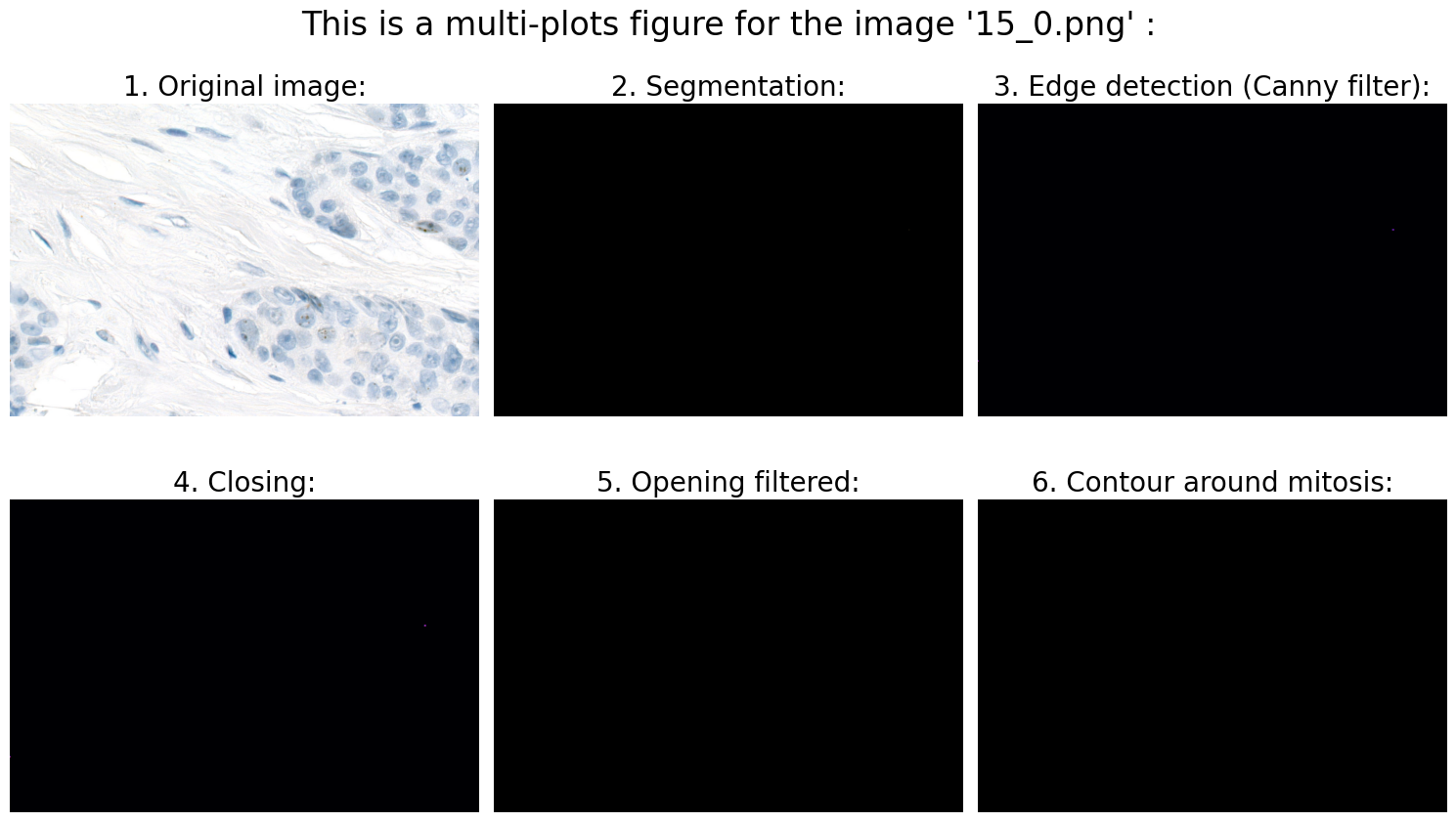
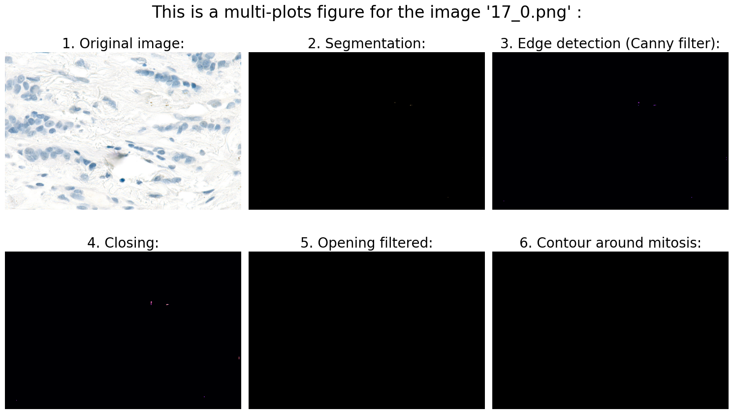
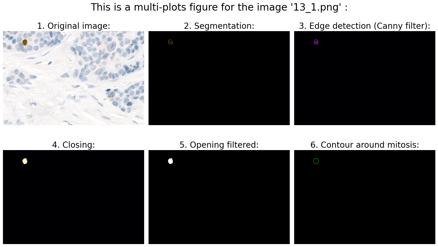
fig_title = "This is a multi-plots figure for the image " + "'" + file_name + "'" + " :"
fig, ((ax1, ax2, ax3), (ax4, ax5, ax6)) = plt.subplots(nrows=2, ncols=3, figsize=(15, 9))
fig.suptitle(fig_title, fontsize=24, y=0.98)
# 6.2 Original image:
ax1.imshow(rgb_img)
ax1.axis('off')
ax1.set_title('1. Original image:', fontsize=20)
# 6.3 Segmentation:
ax2.imshow(result)
ax2.axis('off')
ax2.set_title('2. Segmentation:', fontsize=20)
# 6.4 Edge detection (Canny filter):
ax3.imshow(edges, cmap='magma')
ax3.axis('off')
ax3.set_title('3. Edge detection (Canny filter):', fontsize=20)
# 6.5 Closing:
ax4.imshow(closing, cmap='magma')
ax4.axis('off')
ax4.set_title('4. Closing:', fontsize=20)
# 6.6 Opening filtered:
ax5.imshow(opening_filtered, cmap="gray")
ax5.axis('off')
ax5.set_title('5. Opening filtered:', fontsize=20)
# 6.7 Contour around mitosis:
ax6.imshow(img_contours)
ax6.axis('off')
ax6.set_title('6. Contour around mitosis:', fontsize=20)
# 6.8 Show plt:
fig.subplots_adjust(wspace=0.4, hspace=0.9, top=1.0,
bottom=0.02, left=0.02, right=0.98)
plt.tight_layout()
if answer == "p":
# The accuracy of the result is immediately visible for a large number of images:
total_percentage_of_correct_answers = (correct_solutions / len(files)) * 100
print("")
print("Percentage of correct solutions: ", str(total_percentage_of_correct_answers), "%")'Enter' - display only the results,
'p' - display the results along with an automatic check:
p
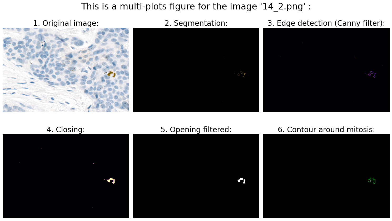
Found mitoses in the image '14_2.png': 2 ✅
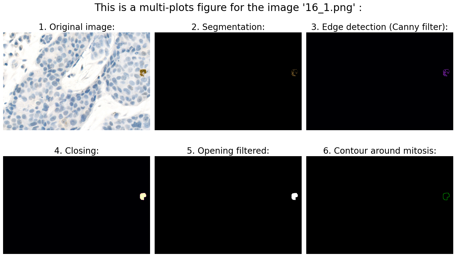
Found mitoses in the image '16_1.png': 1 ✅
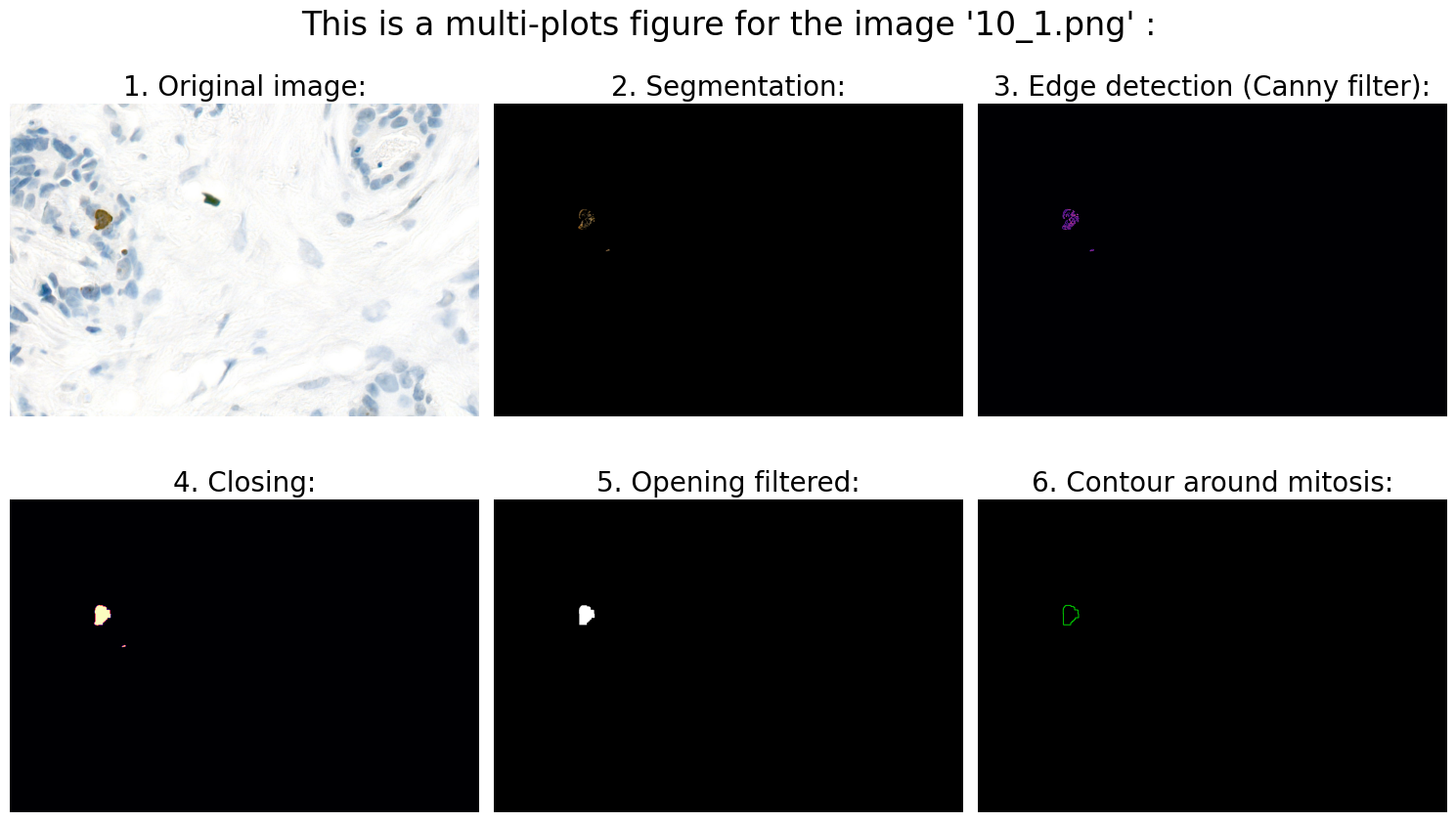
Found mitoses in the image '10_1.png': 1 ✅
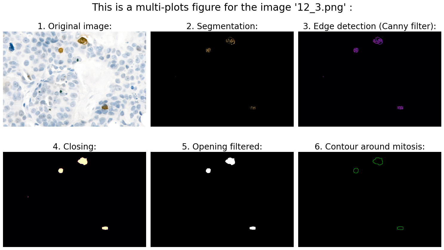
Found mitoses in the image '12_3.png': 3 ✅
Found mitoses in the image '09_2.png': 2 ✅
Found mitoses in the image '15_0.png': 0 ✅
Found mitoses in the image '17_0.png': 0 ✅
Found mitoses in the image '13_1.png': 1 ✅
Found mitoses in the image '08_1.png': 1 ✅
Found mitoses in the image '11_0.png': 0 ✅
Found mitoses in the image '06_3.png': 3 ✅
Found mitoses in the image '04_3.png': 3 ✅
Found mitoses in the image '19_2.png': 2 ✅
Found mitoses in the image '02_2.png': 2 ✅
Found mitoses in the image '20_5.png': 5 ✅
Found mitoses in the image '05_0.png': 0 ✅
Found mitoses in the image '07_2.png': 2 ✅
Found mitoses in the image '01_0.png': 0 ✅
Found mitoses in the image '18_3.png': 3 ✅
Found mitoses in the image '03_1.png': 1 ✅
Percentage of correct solutions: 100.0 %
