RWKV(pronounced as "RwaKuv" (rʌkuv in IPA)) is an RNN with Transformer-level LLM performance, which can also be directly trained like a GPT transformer (parallelizable). And it's 100% attention-free. You only need the hidden state at position t to compute the state at position t+1. You can use the "GPT" mode to quickly compute the hidden state for the "RNN" mode.
So it's combining the best of RNN and transformer - great performance, fast inference, saves VRAM, fast training, "infinite" ctx_len, and free sentence embedding (using the final hidden state).
-
RWKV homepage: https://www.rwkv.com
-
RWKV Discord: https://discord.gg/bDSBUMeFpc (7k+ members)
-
Twitter: https://twitter.com/BlinkDL_AI
-
Online Demo 1(RWKV-6 3B): https://huggingface.co/spaces/BlinkDL/RWKV-Gradio-1
-
Online Demo 2(RWKV-6 7B): https://huggingface.co/spaces/BlinkDL/RWKV-Gradio-2
-
All latest RWKV weights: https://huggingface.co/BlinkDL
-
HF-compatible RWKV weights: https://huggingface.co/RWKV
-
RWKV pip package: https://pypi.org/project/rwkv/
os.environ["RWKV_JIT_ON"] = '1'
os.environ["RWKV_CUDA_ON"] = '0' # if '1' then use CUDA kernel for seq mode (much faster)
from rwkv.model import RWKV                         # pip install rwkv
model = RWKV(model='/fsx/BlinkDL/HF-MODEL/rwkv-4-pile-1b5/RWKV-4-Pile-1B5-20220903-8040', strategy='cuda fp16')

out, state = model.forward([187, 510, 1563, 310, 247], None)   # use 20B_tokenizer.json
print(out.detach().cpu().numpy())                   # get logits
out, state = model.forward([187, 510], None)
out, state = model.forward([1563], state)           # RNN has state (use deepcopy if you want to clone it)
out, state = model.forward([310, 247], state)
print(out.detach().cpu().numpy()) # same result as aboveThe latest architecture of RWKV is v6 , refer to the paper :
- RWKV-5/6 (Eagle/Finch) paper: https://arxiv.org/abs/2404.05892
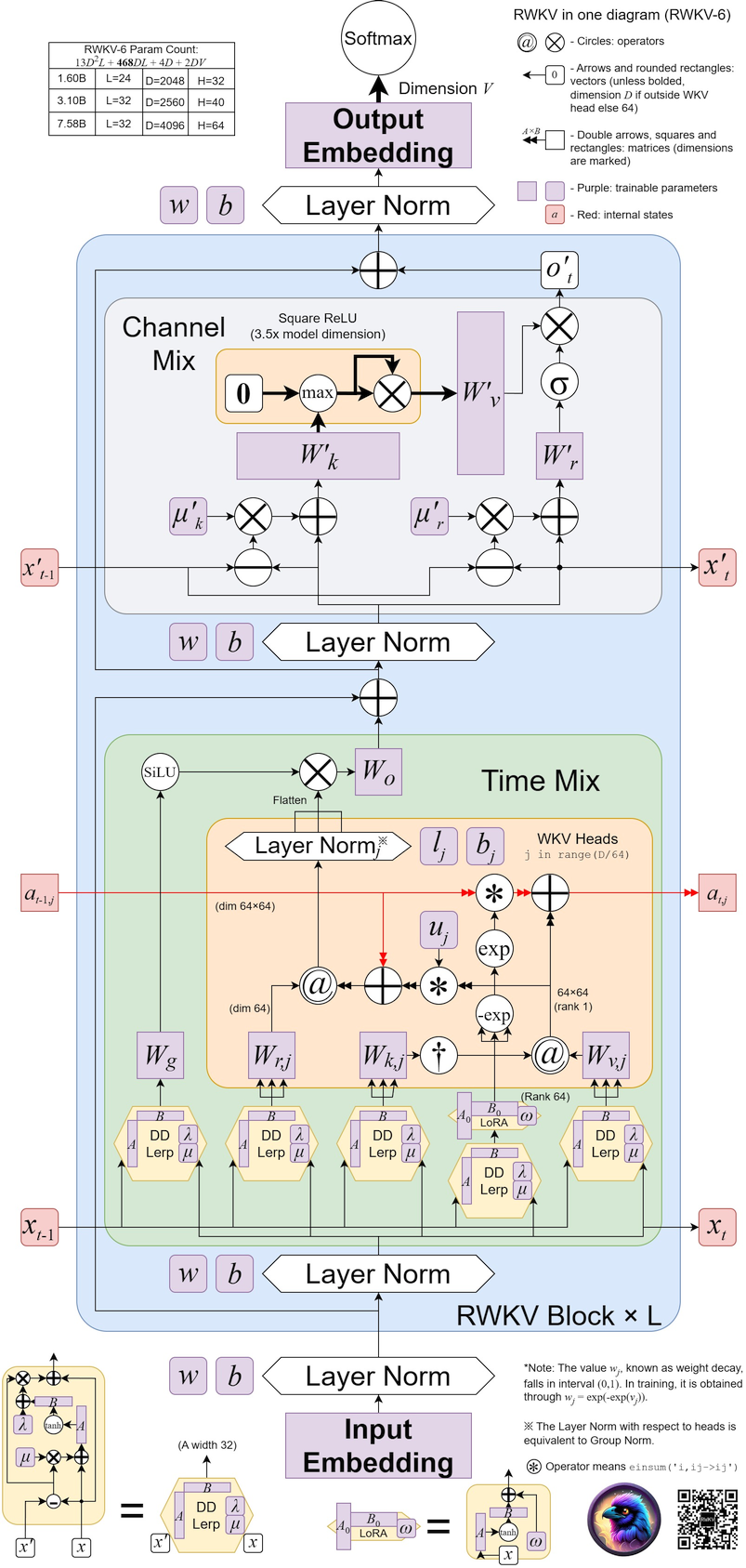
RWKV v6 illustrated:
You can learn about the architecture of RWKV-V5/V6 at the following link:
-
RWKV-6 GPT-mode demo code (with comments and explanations): https://github.com/BlinkDL/RWKV-LM/blob/main/RWKV-v5/rwkv_v6_demo.py
-
RWKV-6 RNN-mode demo in 250 lines(with tokenizer too): https://github.com/BlinkDL/ChatRWKV/blob/main/RWKV_v6_demo.py
-
RWKV v5 in 250 lines (with tokenizer too): https://github.com/BlinkDL/ChatRWKV/blob/main/RWKV_v5_demo.py
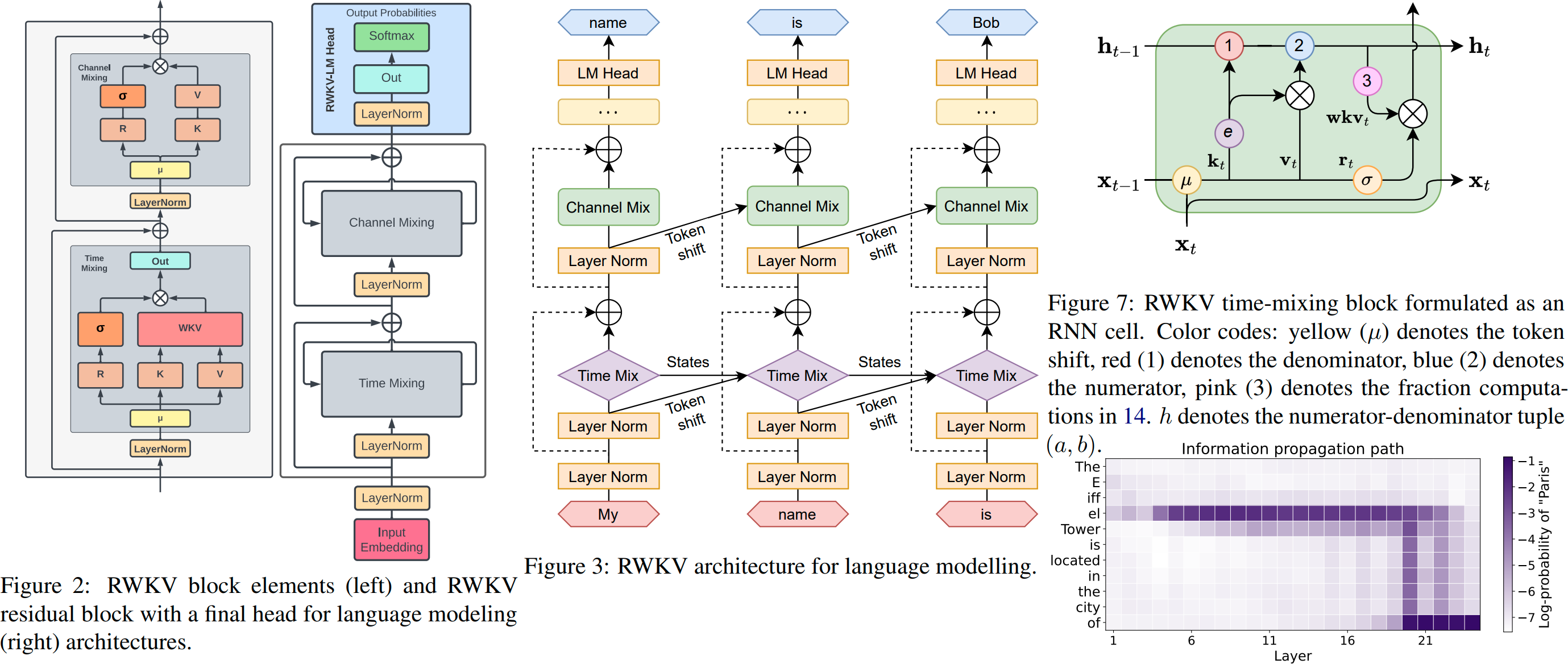
The RWKV community published the first paper on the V4 architecture. See :
- RWKV v4 preprint https://arxiv.org/abs/2305.13048
-
RWKV v4 in 150 lines (model, inference, text generation): https://github.com/BlinkDL/ChatRWKV/blob/main/RWKV_in_150_lines.py
-
RWKV v4 introduction, and in 100 lines of numpy: https://johanwind.github.io/2023/03/23/rwkv_overview.html https://johanwind.github.io/2023/03/23/rwkv_details.html
Due to outdated architecture design, the earlier RWKV architecture (V3/V2/V1) is only used as a historical archive.
RWKV-5 is multi-head and here shows one head. There is also a LayerNorm for each head (hence actually GroupNorm).
Dynamic Mix & Dynamic Decay. Example (do this for both TimeMix & ChannelMix):
TIME_MIX_EXTRA_DIM = 32
self.time_mix_k_w1 = nn.Parameter(torch.empty(args.n_embd, TIME_MIX_EXTRA_DIM).uniform_(-0.01, 0.01))
self.time_mix_k_w2 = nn.Parameter(torch.zeros(TIME_MIX_EXTRA_DIM, args.n_embd))
self.time_mix_v_w1 = nn.Parameter(torch.empty(args.n_embd, TIME_MIX_EXTRA_DIM).uniform_(-0.01, 0.01))
self.time_mix_v_w2 = nn.Parameter(torch.zeros(TIME_MIX_EXTRA_DIM, args.n_embd))
self.time_mix_r_w1 = nn.Parameter(torch.empty(args.n_embd, TIME_MIX_EXTRA_DIM).uniform_(-0.01, 0.01))
self.time_mix_r_w2 = nn.Parameter(torch.zeros(TIME_MIX_EXTRA_DIM, args.n_embd))
self.time_mix_g_w1 = nn.Parameter(torch.empty(args.n_embd, TIME_MIX_EXTRA_DIM).uniform_(-0.01, 0.01))
self.time_mix_g_w2 = nn.Parameter(torch.zeros(TIME_MIX_EXTRA_DIM, args.n_embd))
...
time_mix_k = self.time_mix_k.view(1,1,-1) + (x @ self.time_mix_k_w1) @ self.time_mix_k_w2
time_mix_v = self.time_mix_v.view(1,1,-1) + (x @ self.time_mix_v_w1) @ self.time_mix_v_w2
time_mix_r = self.time_mix_r.view(1,1,-1) + (x @ self.time_mix_r_w1) @ self.time_mix_r_w2
time_mix_g = self.time_mix_g.view(1,1,-1) + (x @ self.time_mix_g_w1) @ self.time_mix_g_w2

xx = self.time_shift(x)
xk = x * time_mix_k + xx * (1 - time_mix_k)
xv = x * time_mix_v + xx * (1 - time_mix_v)
xr = x * time_mix_r + xx * (1 - time_mix_r)
xg = x * time_mix_g + xx * (1 - time_mix_g)
Use parallelized mode to quickly generate the state, then use a finetuned full RNN (the layers of token n can use outputs of all layer of token n-1) for sequential generation.
Important
Before training the RWKV model, ensure that you have set up the appropriate environment.
For reference, use python 3.10, torch==1.13.1+cu117, cuda 11.7.1.
For best performance, use python 3.10, torch 2.1.2+cu121 (or latest), cuda 12.3+, latest deepspeed, but keep pytorch-lightning==1.9.5
reference:
pip install torch==1.13.1+cu117 --extra-index-url https://download.pytorch.org/whl/cu117
pip install pytorch-lightning==1.9.5 deepspeed==0.7.0 wandb ninja

best performance:
pip install torch --upgrade --extra-index-url https://download.pytorch.org/whl/cu121
pip install pytorch-lightning==1.9.5 deepspeed wandb ninja --upgrade# mkdir -p data
# wget --continue -O data/minipile.idx https://huggingface.co/datasets/BlinkDL/minipile-tokenized/resolve/main/rwkv_vocab_v20230424/minipile.idx
# wget --continue -O data/minipile.bin https://huggingface.co/datasets/BlinkDL/minipile-tokenized/resolve/main/rwkv_vocab_v20230424/minipile.bin
cd RWKV-v5/
./demo-training-prepare.sh
./demo-training-run.sh
(you may want to log in to wandb first)
Your loss curve should look almost exactly the same as this, with the same ups and downs (if you use the same bsz & config):
You can run your model using https://pypi.org/project/rwkv/ (use "rwkv_vocab_v20230424" instead of "20B_tokenizer.json")
Follow the steps to prepare your training dataset.
- Collect jsonl data
Organize your data into JSONL files, refer to the format:
# Single-turn dialogue
{“text”: “User: Question\n\nAssistant: Answer”}

# Multi-turn dialogue
 {“text”: “User: First question\n\nAssistant: First answer\n\nUser: Second question\n\nAssistant: Second answer”}

# Material-based Q&A
{“text”: “Instruction: Directive\n\nInput: Material\n\nResponse: Answer”}

# Content generation/continuation
 {“text”: “Transform the content of each article into one line of JSONL, even if it is a novel of one million words.”} or {“text”: “Title\n\nMain text content”}
- Convert jsonl data to binidx
Use RWKV-v5/make_data.py to prepare binidx data ( suitable for finetuning RWKV-World models) from your jsonl file , and compute "--my_exit_tokens" and "--magic_prime".
usage:
python make_data.py demo.jsonl 3 4096This will:
- shuffle & duplicate demo.jsonl (for 3 epochs, good for finetuning)
- load jsonl and tokenize
- convert
demo.jsonlto binidx data,save asdemo.bin&demo.idx - compute "
magic_prime" for ctxlen 4096
Tip
simple SFT jsonl data: repeat your SFT data 3 or 4 times in make_data.py. more repetition leads to overfitting.
advanced SFT jsonl data: repeat your SFT data 3 or 4 times in your jsonl (note: make_data.py will shuffle all jsonl items) => add some base data (such as slimpajama) to your jsonl => and only repeat 1 times in make_data.py.
Tip
All training parameters can be modified in demo-training-run.sh. Modifying training parameters will affect the training process and model training effect.
Parameters that must be modified
--load_model # Path to base RWKV model
--proj_dir # Path to save the trained model
--data_file # Path to the data file, no need `.bin` or `.idx` for binidx data , just the filename
--n_layer # according to the Size of the model
--n_embd # according to the Size of the model
--my_exit_tokens # tokens number of the training data
--magic_prime # Prime number related to my_exit_tokens / ctx_len--n_layerand--n_embdneed to be adjusted according to the Size of the model:
| RWKV Model Size | n_layer | n_embd |
|---|---|---|
| 0.1B | 12 | 768 |
| 0.4B | 24 | 1024 |
| 1.5B | 24 | 2048 |
| 3B | 32 | 2560 |
| 7B | 32 | 4096 |
--my_exit_tokens" and "--magic_primeshould be computed when usingRWKV-v5/make_data.py. If you get a ready-made bindix dataset, you can manually calculate its--magic_primeparameter :
Note
--my_exit_tokens & --magic_prime
The "epoch" in train.py is "mini-epoch" (not real epoch. only for convenience), and 1 mini-epoch = 40320 * ctx_len tokens.
For example, if your binidx has 1498226207 tokens and ctxlen=4096, set "--my_exit_tokens 1498226207" (this will override epoch_count), and it will be 1498226207/(40320 * 4096) = 9.07 miniepochs. The trainer will auto-exit after "--my_exit_tokens" tokens.
Set "--magic_prime" to the largest 3n+2 prime smaller than datalen/ctxlen-1 (= 1498226207/4096-1 = 365776), which is "--magic_prime 365759" in this case.
Parameters can keep the default value
--my_testing x060 # base model type, x060 => rwkv-6.0 , x052 => rwkv-5.2
--ctx_len 512 # Maximum context length, if modifying this value, remember to also compute and modify --magic_prime
--my_pile_stage 3 # Set to 1 for generating rwkv-init.pth,  3 for training
--epoch_count 999999 # Total training epochs, will be overridden by --my_exit_tokens parameter
--epoch_begin 0 # Initial training epoch, indicating to start loading from the N-th epoch
--my_exit_tokens 1498226207 # Stop training after reaching the specified number of tokens, depending on your dataset size
--magic_prime 2926181 # Prime number related to my_exit_tokens / ctx_len, refer to previous text for specific calculations
--num_nodes 1 # Number of nodes
--micro_bsz 16 # Micro batch size (batch size per GPU), increasing it may be better but takes more VRAM
--pre_ffn 0 # Replace the first att layer with ffn,default 0 (sometimes 1 better)
--head_qk 0 # Usually keep the default value 0 (off)
--lr_init 1e-5 # Initial learning rate, use smaller values like 1e-5 for fine-tuning
--lr_final 1e-5 # Final learning rate, use smaller values like 1e-5 for fine-tuning
--warmup_steps 10 # Warm-up steps, try 50 if loading a model
--beta1 0.9 # Beta1 parameter of Adam optimizer, usually 0.9
--beta2 0.99 # Beta2 parameter of Adam optimizer, use 0.999 when nearing convergence
--adam_eps 1e-8 # Epsilon parameter of Adam optimizer, usually 1e-8
--my_pile_edecay 0 # Pile decay setting, usually set to 0
--data_type binidx # Format of training  data, supports "utf-8", "utf-16le", "numpy", "binidx", "dummy", "wds_img", "uint16"
--vocab_size 65536 # Vocabulary size, default 65536, setting to 0 means the model will determine the vocabulary size automatically
--weight_decay 0.001 # Weight decay, default 0.001, can try 0.1 / 0.01 / 0.001
--epoch_save 10 # Save the trained model every 10 "miniepochs" ,mind your storage space when set to smaller.
--head_size_a 64 # Size of attention head, default 64, can try increasing this value for larger training models
--accelerator gpu # Type of accelerator, though options are cpu/gpu, currently cpu does not support training
--devices 1 # 1 for single GPU, fill in the number of GPUs for multiple cards
--precision bf16 # Training precision, default bf16, supports "fp32", "tf32", "fp16", "bf16"
--strategy deepspeed_stage_2 # Training strategy parameter for lightning, default deepspeed_stage_2
--grad_cp 1 # Gradient accumulation steps, 1 => slower training & save VRAM; 0 => faster & need more VRAM
--enable_progress_bar True # Enable progress bar
--ds_bucket_mb 2 # Deep learning speed size, set to 2 for consumer GPUs,200 for A100 / H100 (affects speed & vram usage)Rename the base checkpoint in your model folder to rwkv-init.pth, run demo-training-run.sh:
cd RWKV-v5/
./demo-training-prepare.sh
./demo-training-run.sh
(you may want to log in to wandb first)Currently unoptimized implementation, takes same vram as full SFT .
Modify parameters in demo-training-run.sh:
--train_type "states"
--load_partial 1
--lr_init 1 # (yes, use very high LR)
--lr_final 0.01
--warmup_steps 10
use rwkv 0.8.26+ to auto-load the trained "time_state"
When you train RWKV from scratch, try my initialization for best performance. Check generate_init_weight() of src/model.py:
emb.weight => nn.init.uniform_(a=-1e-4, b=1e-4)
(Note ln0 of block0 is the layernorm for emb.weight)
head.weight => nn.init.orthogonal_(gain=0.5*sqrt(n_vocab / n_embd))

att.receptance.weight => nn.init.orthogonal_(gain=1)
att.key.weight => nn.init.orthogonal_(gain=0.1)
att.value.weight => nn.init.orthogonal_(gain=1)
att.gate.weight => nn.init.orthogonal_(gain=0.1)
att.output.weight => zero

att.ln_x.weight (groupnorm) => ((1 + layer_id) / total_layers) ** 0.7

ffn.key.weight => nn.init.orthogonal_(gain=1)
ffn.value.weight => zero
ffn.receptance.weight => zero
Important
If you are using positional embedding, maybe it's better to remove block.0.ln0 and use default initialization for emb.weight instead of my uniform_(a=-1e-4, b=1e-4)
Tip
Tips for small model / small data: When I train RWKV music models, I use deep & narrow (such as L29-D512) dimensions, and apply wd and dropout (such as wd=2 , dropout=0.02).
Note RWKV-LM dropout is very effective - use 1/4 of your usual value.
-
Train RWKV-6: use /RWKV-v5/ , and add
--my_testing "x060"todemo-training-prepare.shanddemo-training-run.sh. -
Simple inference for RWKV-5: https://github.com/BlinkDL/ChatRWKV/blob/main/RWKV_v5_demo.py
-
Simple inference for RWKV-6: https://github.com/BlinkDL/ChatRWKV/blob/main/RWKV_v6_demo.py
-
lm_eval: https://github.com/BlinkDL/ChatRWKV/blob/main/run_lm_eval.py
-
chat demo for developers: https://github.com/BlinkDL/ChatRWKV/blob/main/API_DEMO_CHAT.py
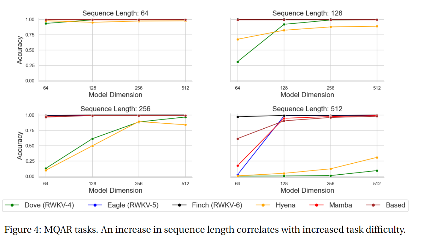
MQAR for non-transformer architecture:
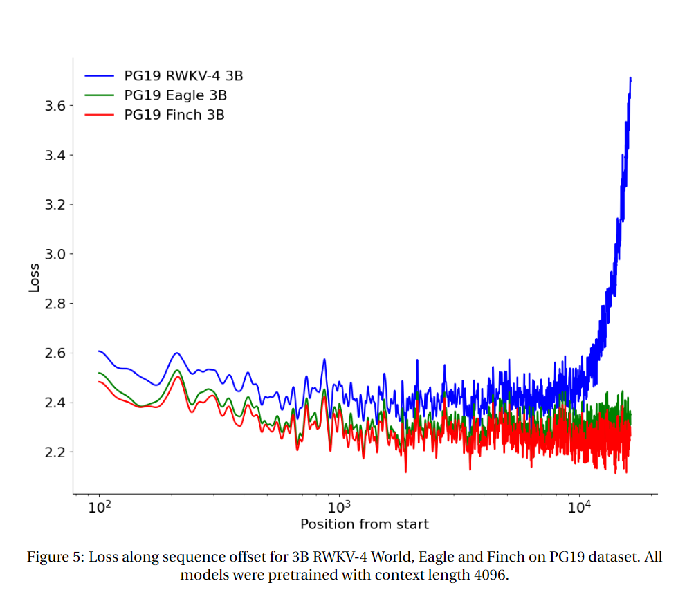
Long Context Experiments for RWKV v4/v5/v6 :
English and Multilingual Benchmarks for RWKV-6 7B:
Uncheatable Eval (testing LLMs on real-time, newly generated data) for RWKV-6 7B:
-
All (300+) RWKV projects: https://github.com/search?o=desc&q=rwkv&s=updated&type=Repositories
-
Vision RWKV: https://github.com/OpenGVLab/Vision-RWKV
-
Diffusion RWKV: https://github.com/feizc/Diffusion-RWKV
-
RWKV Runner GUI: https://github.com/josStorer/RWKV-Runner with one-click install and API
-
Ai00-server: https://github.com/cgisky1980/ai00_rwkv_server Fastest WebGPU inference (nVidia/AMD/Intel), supports rwkv5 & rwkv6
-
web-rwkv: https://github.com/cryscan/web-rwkv backend for ai00_rwkv_server
-
rwkv.cpp:https://github.com/saharNooby/rwkv.cpp Fast CPU/cuBLAS/CLBlast inference: int4/int8/fp16/fp32, supports rwkv5
-
faster-rwkv: https://github.com/daquexian/faster-rwkv supports rwkv5
-
MLC LLM supports rwkv5: mlc-ai/mlc-llm#1275
-
Infctx trainer: https://github.com/RWKV/RWKV-infctx-trainer
-
LoRA finetuning: https://github.com/Blealtan/RWKV-LM-LoRA
-
Digital Assistant with RWKV: https://github.com/TheRamU/Fay
-
rwkv-cpp-cuda: https://github.com/harrisonvanderbyl/rwkv-cpp-cuda Fast GPU inference with cuda/amd/vulkan
-
A cool paper (Spiking Neural Network) using RWKV: https://github.com/ridgerchu/SpikeGPT
RWKV is inspired by Apple's AFT (https://arxiv.org/abs/2105.14103).
Moreover it's using a number of my tricks, such as:
-
SmallInitEmb: https://github.com/BlinkDL/SmallInitEmb (applicable to all transformers) which helps the embedding quality, and stabilizes Post-LN (which is what I am using).
-
Token-shift: https://github.com/BlinkDL/RWKV-LM#token-shift-time-shift-mixing (applicable to all transformers), especially helpful for char-level models.
-
Head-QK: https://github.com/BlinkDL/RWKV-LM#the-head-qk-trick-learning-to-copy-and-avoid-tokens (applicable to all transformers). Note: it's helpful, but I disabled it in the Pile model to keep it 100% RNN.
-
Extra R-gate in the FFN (applicable to all transformers). I am also using reluSquared from Primer.
-
Better initilization: I init most of the matrices to ZERO (see RWKV_Init in https://github.com/BlinkDL/RWKV-LM/blob/main/RWKV-v2-RNN/src/model.py).
-
You can transfer some parameters from a small model to a large model (note: I sort & smooth them too), for faster and better convergence (see https://www.reddit.com/r/MachineLearning/comments/umq908/r_rwkvv2rnn_a_parallelizable_rnn_with/).
-
My CUDA kernel: https://github.com/BlinkDL/RWKV-CUDA to speedup training.


