Data from Peter and Rosemary Grant research of Darwin's finches on Galápagos island of Daphne Major.
First let's see how the beak depth (the distance, top to bottom, of a closed beak) of the finch species Geospiza scandens has changed over time.
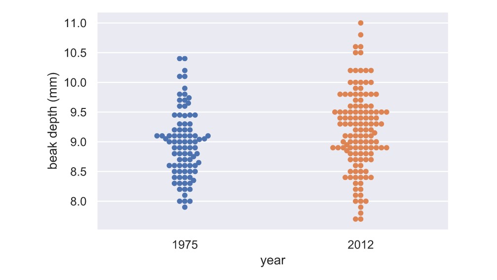
_ = sns.swarmplot(x='year', y='beak_depth', data=df)It's hard to see if there is a clear difference between the 1975 and 2012 data set. But, it appears as the mean of the 2012 dataset might be slightly higher, and it might have a bigger variance.
x_1975, y_1975 = ecdf(bd_1975)
x_2012, y_2012 = ecdf(bd_2012)

_ = plt.plot(x_1975, y_1975, marker='.', linestyle='none')
_ = plt.plot(x_2012,y_2012, marker='.', linestyle='none')
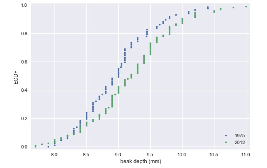
The differences are much clearer in the ECDF. The mean is larger in the 2012 data, and the variance does appear larger as well.
# the difference of the sample means: mean_diff
mean_diff = diff_of_means(bd_2012,bd_1975)

# bootstrap replicates of means
bs_replicates_1975 = draw_bs_reps(bd_1975, np.mean, size=10000)
bs_replicates_2012 = draw_bs_reps(bd_2012, np.mean, size=10000)

# samples of difference of means: bs_diff_replicates
bs_diff_replicates = bs_replicates_2012 - bs_replicates_1975

# 95% confidence interval: conf_int
conf_int = np.percentile(bs_diff_replicates, [2.5, 97.5])

print('difference of means =', mean_diff, 'mm')
print('95% confidence interval =', conf_int, 'mm')

>>> difference of means = 0.22622047244094645 mm
>>> 95% confidence interval = [0.05633521 0.39190544] mmThe ECDF and determination of the confidence interval make it pretty clear that the beaks of G. scandens on Daphne Major have gotten deeper. But is it possible that this effect is just due to random chance? In other words, what is the probability that we would get the observed difference in mean beak depth if the means were the same?
combined_mean = np.mean(np.concatenate((bd_1975, bd_2012)))

# Shift the samples
bd_1975_shifted = bd_1975 - np.mean(bd_1975) + combined_mean
bd_2012_shifted = bd_2012 - np.mean(bd_2012) + combined_mean

# Bootstrap replicates of shifted data sets
bs_replicates_1975 = draw_bs_reps(bd_1975_shifted, np.mean, size=10000)
bs_replicates_2012 = draw_bs_reps(bd_2012_shifted, np.mean, size=10000)

bs_diff_replicates = bs_replicates_2012 - bs_replicates_1975

# p-value
p = np.sum(bs_diff_replicates >= mean_diff) / len(bs_diff_replicates)

print('p =', p)

>>> p = 0.0034
p-value of 0.0034 suggests that there is a statistically significant difference.
That means, the beak length have changed over the course of 37 years.
# scatter plot of 1975 data
_ = plt.plot(bl_1975, bd_1975, marker='.', linestyle='None', color='blue', alpha=0.5)

# scatter plot of 2012 data
_ = plt.plot(bl_2012, bd_2012, marker='.', linestyle='None', color='red', alpha=0.5)

plt.show()
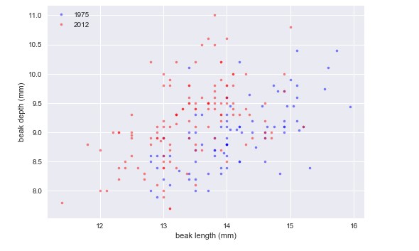
Looking at the plot, we see that beaks got deeper and a bit shorter. So, it does not look like the beaks kept the same shape; they became shorter and deeper.
Code can be found here
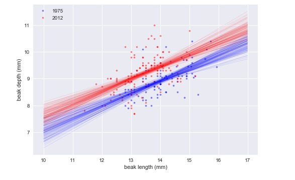
It looks like they have the same slope, but different intercepts.
1975: slope = 0.4652051691605937 conf int = [0.33310645 0.58996223]
1975: intercept = 2.3908752365842263 conf int = [0.60754109 4.21248022]
2012: slope = 0.462630358835313 conf int = [0.33060855 0.60024108]
2012: intercept = 2.9772474982360198 conf int = [1.15365093 4.72831245]
The slope was the same in 1975 and 2012, suggesting that for every millimeter gained in beak length, the birds gained about half a millimeter in depth in both years. However, if we are interested in the shape of the beak, we want to compare the ratio of beak length to beak depth.
# length-to-depth ratios
ratio_1975 = bl_1975/bd_1975
ratio_2012 = bl_2012/bd_2012

# means
mean_ratio_1975 = np.mean(ratio_1975)
mean_ratio_2012 = np.mean(ratio_2012)

# bootstrap replicates of the means
bs_replicates_1975 = draw_bs_reps(ratio_1975, np.mean, size=10000)
bs_replicates_2012 = draw_bs_reps(ratio_2012, np.mean, size=10000)

# 99% confidence intervals
conf_int_1975 = np.percentile(bs_replicates_1975, [0.5,99.5])
conf_int_2012 = np.percentile(bs_replicates_2012, [0.5,99.5])
1975: mean ratio = 1.5788823771858533 conf int = [1.55668803 1.60073509] 2012: mean ratio = 1.4658342276847767 conf int = [1.44363932 1.48729149]
It is impossible to say if this is a real effect or just due to noise without computing a p-value.


