hmctdm
hmctdm is open source package for bayesian estimation of PK parameters using stan in R. The main function, hmctdmrest() , can estimate individual PK parameters. below is a drug that can be estimate from the function:
- Amikacin (IV)
- Vancomycin (IV)
- Theophiline (Oral)
- Phenytoin (Oral)
The pharmacokinetic model was implemented from the PKS program.
Installation
You can install development version from github by executing the following code in R console.
install.packages("devtools")
devtools::install_github("sikso1897/hmctdm")
hmctdm relies on the following software & packages.
- Stan is an open source probabilistic programing language designed primarily to do Bayesian data analysis
- Torsten is a collection of Stan functions to facilitate analysis of pharmacometric data.
- Mrgsolve is model implementation and ordinary differential equation solver
Please refer to the installation guide of these programs
Example
library(cmdstanr)
library(hmctdm)
1) set cmdstan path
HOME_TORSTEN <- "path/to/torsten"
suppressMessages(set_cmdstan_path(file.path(HOME_TORSTEN, 'cmdstan')))
2) bring data set
checking the sample data and bring data of type data.frame or tibble by format of sample data.
sample_data <- hmctdmr::get_sample_data(drug="amikacin")
sample_data

#   ID time evid amt cmt ss ii addl rate SEX AGE       WT       HT      SCR      DV
# 1  1    0    1 500   1  0  0    0 1000   1  79 43.97928 155.7253 1.072065  0.0000
# 2  1    1    0   0   1  0  0    0    0   1  79 43.97928 155.7253 1.072065 28.5206
3) estimate
hmctdm <- hmctdmr::hmctdmrest(drug="amikacin", data="your_data_set")
print(hmctdm)
# Model executable is up to date!
# Running MCMC with 4 sequential chains...
# Chain 1 finished in 0.6 seconds.
# Chain 2 finished in 0.6 seconds.
# Chain 3 finished in 0.5 seconds.
# Chain 4 finished in 0.5 seconds.
# All 4 chains finished successfully.
# Mean chain execution time: 0.6 seconds.
# Total execution time: 3.0 seconds.
# Building amikacin ... done.
# Building amikacin ... (waiting) ...
# done.
# Status: Sample
# Drug: Amikacin
# Stan sample option:
# # A tibble: 1 × 3
# option dir compile
# <chr> <chr> <chr>
# 1 stan_model_option .../stanc TRUE
# Stan model option:
# # A tibble: 1 × 7
# option chains thin iter_warmup iter_sampling output_dir adapt_delta
# <chr> <chr> <chr> <chr> <chr> <chr> <chr>
# 1 stan_sample_option 4 1 2500 2500 .../stan_output 0.95
# Prior Information:
# # A tibble: 6 × 2
# parameter value
# <chr> <dbl>
# 1 Prior_CL_NR 0.0417
# 2 Prior_VD_NR 0.27
# 3 Prior_CL_SLOPE 0.815
# 4 Prior_CL_NR_omega 0.246
# 5 Prior_VD_NR_omega 0.294
# 6 Prior_CL_SLOPE_omega 0.385
# Estimated PK Parameters:
# # A tibble: 5 × 10
# variable mean median sd mad q5 q95 rhat ess_bulk ess_tail
# <chr> <dbl> <dbl> <dbl> <dbl> <dbl> <dbl> <dbl> <dbl> <dbl>
# 1 CL_NR 0.0431 0.0419 0.0108 0.0104 0.0277 0.0626 1.00 6045. 4133.
# 2 VD_NR 0.336 0.335 0.0556 0.0554 0.247 0.429 1.00 6087. 5655.
# 3 CL_SLOPE 0.925 0.853 0.382 0.330 0.450 1.64 1.00 4353. 3045.
# 4 CL 2.00 1.85 0.778 0.673 1.03 3.45 1.00 4338. 3091.
# 5 VD 14.8 14.7 2.44 2.44 10.9 18.9 1.00 6087. 5655.
# Estimated Concentration:
# ID time evid amt cmt ss ii addl rate SEX AGE WT LBW HT SCR CrCL DV cHat
# 1 1 0 1 500 1 0 0 0 1000 1 79 43.97928 43.97928 155.7253 1.072065 33.95356 0.0000 0.00000
# 2 1 1 0 0 1 0 0 0 0 1 79 43.97928 43.97928 155.7253 1.072065 33.95356 28.5206 30.65465
# Individual Data:
# ID SEX AGE WT LBW HT SCR CrCL CL_NR VD_NR CL_SLOPE CL VD
# 1 1 1 79 43.97928 43.97928 155.7253 1.072065 33.95356 0.0418793 0.334881 0.853423 1.85247 14.72785
4) predict concentration
The concentration at the new time point is predicted using the mrgsolve model, which is the same as the pharmacokinetic model used for estimation. The result contains an mrgsolve model object.
hmctdm <- hmctdmr::hmctdmrest(drug="amikacin", data="your_data_set")

hmctdm$mrgmod
# ---------------  source: amikacin.cpp  ---------------

#   project: ...inst/mrgsolve
#   shared object: amikacin-so-22cda12102f

#   time:          start: 0 end: 30 delta: 0.5
#                  add: <none>

#   compartments:  CENT [1]
#   parameters:    WT LBW CLCR CL_NR CL_SLOPE VD_NR
#                  VD_SLOPE UNIT_CL [8]
#   captures:      CL VD IPRED [3]
#   omega:         0x0
#   sigma:         0x0

#   solver:        atol: 1e-08 rtol: 1e-05 maxsteps: 20k
# ------------------------------------------------------

mrgmod <- hmctdm$mrgmod %>%
  mrgsolve::ev(amt=1000) %>%
  mrgsolve::mrgsim(end=48, delta=0.5)

mrgmod
# Model:  amikacin
# Dim:    98 x 19
# Time:   0 to 48
# ID:     1
#     ID time evid  amt cmt ss ii addl rate SEX AGE    WT    HT   LBW   SCR    AUC    CL    VD IPRED
# 1:   1  0.0    0    0   0  0  0    0    0   1  79 43.98 155.7 43.98 1.072   0.00 1.651 14.75  0.00
# 2:   1  0.0    1 1000   1  0  0    0    0   1  79 43.98 155.7 43.98 1.072   0.00 1.651 14.75 67.79
# 3:   1  0.5    0    0   0  0  0    0    0   1  79 43.98 155.7 43.98 1.072  32.97 1.651 14.75 64.10
# 4:   1  1.0    0    0   0  0  0    0    0   1  79 43.98 155.7 43.98 1.072  64.14 1.651 14.75 60.61
# 5:   1  1.5    0    0   0  0  0    0    0   1  79 43.98 155.7 43.98 1.072  93.61 1.651 14.75 57.32
# 6:   1  2.0    0    0   0  0  0    0    0   1  79 43.98 155.7 43.98 1.072 121.48 1.651 14.75 54.20
# 7:   1  2.5    0    0   0  0  0    0    0   1  79 43.98 155.7 43.98 1.072 147.84 1.651 14.75 51.25
# 8:   1  3.0    0    0   0  0  0    0    0   1  79 43.98 155.7 43.98 1.072 172.76 1.651 14.75 48.46
This object can use generic functions. More details can be found here. below is generic functions example.
mrgmod %>%
  mrgsolve::plot(IPRED ~ time)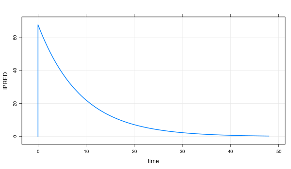
5) usage for get recommended dose
using the mrgsolve model in which the parameters estimated above are used, various dosage regimens can be simulated and drug titration regimens can be obtained. (get_recommended_dose, get_b_cp)
each parameter used in the function is calculated based on the steady state. In order to know the steady state of the current regimens, you can obtain the result in the steady state by using the following code.
simdata <- hmctdm$mrgmod %>%
            mrgsolve::ev(amt=200, ii=12, addl=4, ss=1) %>%  # current regimen with ss=1 added.
            mrgsolve::mrgsim(end=48, delta=0.5)
you can see the result with the code below and the result contains the concentration and AUC for each hour here.
# data.table
print(simdata@data) # or simdata

# plot
simdata %>%
  mrgsolve::plot(IPRED ~ time)
creating event(regimens) is described in the mrgsolve specific section below, and more detailed information can be found in mregsolve repository.
5-1) get_recommended_dose
get_recommended_dose calculates the appropriate dose by using the following formula to obtain the target result.
paramerters are mode, target, current_dose, current_status, non-linear pk parameters
-
modeis what you want to target.AUCis steady-stateCpis steady-state concetrationb_Cpis average steady-state concentration
-
targetis the desired value -
current_doseis dosage of current regimen -
current_statusis if the current regimen is maintained, the value at target timesimdata <- hmctdm$mrgmod %>% mrgsolve::ev(amt=200, ii=12, addl=4, ss=1) %>% # current regimen with ss=1 added. mrgsolve::mrgsim(end=48, delta=0.5)
-
non-linear pk params- if
modeis average steady-state concentration(=b_Cp), the following parameters are required. (Vmax,CL_R,Km,F,tau)
- if
5-2) Stedy-state concentration
5-3) Steady-state AUC
5-4) Average steady-state concentration
get_recommended_dose(mode=mode, target=target,
                      current_dose=current_dose,
                      current_status=current_status,
                      ...)
# ... is non-linear pk params. if mode use b_Cp, have to insert non-linear pk params like Vmax mentioned at above phrase
Specific
1) mrgsolve specific
this session is introduction to mrgsolve model object, focusing on the simulation used in hcmtdmr. if you want to know more details, for more information at mregsolve repository.
# how to get mrgsolve model object at result
est <- hmctdmr::hmctdmrest(...)
mrgmod <- est$mrgmod

# or if you want to get default mrgsolve model in package
mrgmod <- hmctdmr::get_mrgmod(drug="drug") # drug, amikacin, vanocomycin ...
the overall process of using mrgsolve in a package is as follows step. step-1) define a pharmacokinetic model, step-2) enter patient information in the model, step-3) generate a dosing event. step-4) Run the simulation. the package returns an object that has progressed up to step-2.
information about model details can be obtained by printing the object.
print(mrgmod)# --------------- source: amikacin.cpp ---------------
# project: ...inst/mrgsolve
# shared object: amikacin-so-22cda12102f
# time: start: 0 end: 30 delta: 0.5
# add: <none>
# compartments: CENT [1]
# parameters: WT LBW CLCR CL_NR CL_SLOPE VD_NR
# VD_SLOPE UNIT_CL [8]
# captures: CL VD IPRED [3]
# omega: 0x0
# sigma: 0x0
# solver: atol: 1e-08 rtol: 1e-05 maxsteps: 20k
# ------------------------------------------------------step-3 and 4 provide simulations that allow users to experiment with different drug regimens. (to improve regimen) it proceeds in the form of example-4 (prediction).
mrgmod <- hmctdm$mrgmod %>%
  mrgsolve::ev(amt=1000) %>%
  mrgsolve::mrgsim(end=48, delta=0.5)
1-1) event(ev)
events may be observations, doses, or other type events.
-
timeorTIME: states the time of the data record -
evidorEVID: the event id indicator. evid can take the values:- 0 = observation record
- 1 = dosing event (bolus or infusion)
- 2 = other type event, with solver stop and restart
- 3 = system reset
- 4 = reset and dose
- 8 = replace the amount in the compartment with amt
-
amtorAMT: the dose amount (if evid==1) -
cmtorCMT: the dosing compartment number. This may also be a character value naming the compartment name. The compartment number must be consistent with the number of compartments in the model for dosing records (evid==1).
For observation records, a cmt value of 0 is acceptable. Use a negative compartment number withevid2 to turn a compartment off. -
rateorRATE: if non-zero and evid=1 or evid=4, implements a zero-order infusion of duration F_CMT*amt/rate, where F_CMT is the bioavailability fraction for the dosing compartment. Use rate = -1 to model the infusion rate and rate = -2 to model the infusion duration. -
iiorII: inter-dose interval; ii=24 means daily dosing when the model time unit is hours -
addlorADDL: additional doses; a non-zero value in addl requires non-zero ii on the same record -
ssorSSsteady state indicator; use 1 to implement steady-state dosing; 0 otherwise. mrgsolve also recognizes dosing records wheress=2. This allows combination of different steady state dosing regimens under linear kinetics (e.g. 10 mg QAM and 20 mg QPM daily to steady state).
# example-1.
event <- mrgsolve::ev(amt=100, ii=24, addl=3)

# example-2. multiple event ( 250 mg every 8 hours for 12 total doses )
event <- mrgsolve::expand.ev(ID=1:3, amt=250, ii=8, addl=11)

# example-3. dose as a 2-hour infusion into the second compartment use
event <- mrgsolve:: expand.ev(ID=1:3, amt=250, rate=125, ii=8, addl=11, cmt=2)
mrgmod %>% ev(event)1-2) simulate (mrgsim)
mrgsim is used to simulate from a model, it by default returns an object with class mrgsims.
out <- mrgsim(mod, ..., output = "df")

# or using pipeline
out <- mrgmod %>% mrgsim(...)
2) hmctdm specific
hmctdmrest takes the following parameters:
hmctdmrest <- function(drug=NULL,
                    data=NULL,
                    prior=NULL,
                    stan_model_option=NULL,
                    stan_sample_option=NULL){
                    ...
}
hmctdmrest can be given the following parameters:
2-1) drug
- amikacin
- vancomycin
- theophiline
- phenytoine
2-2) data
checking the sample data as using get_sample_data and bring data of type data.frame or tibble by format of sample data.
sample_data <- hmctdmr::get_sample_data(drug="amikacin")
sample_data

#   ID time evid amt cmt ss ii addl rate SEX AGE       WT       HT      SCR      DV
# 1  1    0    1 500   1  0  0    0 1000   1  79 43.97928 155.7253 1.072065  0.0000
# 2 1 1 0 0 1 0 0 0 0 1 79 43.97928 155.7253 1.072065 28.5206IDis subject indicator.time,evid,amt,cmt,ss,ii,addl,rateare described in the mrgsolve specific section..SEX,AGE,WT,HTare demographics. (sex, age, weight, height)SCR,DVis serum creatinine and concentration.
2-3) prior
It can be changed by passing the prior parameter in the list.
# example

hmctdmr::get_default_prior(drug="amikacin")
# $Prior_CL_NR
# [1] 0.0417

# $Prior_VD_NR
# [1] 0.27

# $Prior_CL_SLOPE
# [1] 0.815

# $Prior_CL_NR_omega
# [1] 0.2462207

# $Prior_VD_NR_omega
# [1] 0.2935604

# $Prior_CL_SLOPE_omega
# [1] 0.3852532


hmctdm <- hmctdmr::hmctdmrest(
                    drug="amikacin",
                    data="your_data_set",
                    prior=list(
                      CL_NR=0.5,
                      CL_NR_omega=0.3
                    ))
}
2-4) stan_model_option
stan_model_option is an option for creating a new CmdStanModel object from a file containing a Stan program. More information on the options can be found here
2-5) stan_sample_option
stan_sample_option is option of $sample() method CmdStanModel objcet runs the default MCMC algorithm in CmdStan (algorithm = hmc, engine=nuts). More information on the options can be found here
Development
hmctdm is under development. Your feedback for additional feature requests or bug reporting is welcome. Contact us through the issue tracker.