-
CUDA 11.0
-
Anaconda: Python 3.7
-
Tensorflow 1.15.0
Downloaded original author's repo to study the code
Trying to build the pre-trained network following the repo linked in the paper.
PS: almost all code in this directory are from the linked GitHub repo above. I checked out that folder only as svn and copied it here for easy testing. test.py contains the code I put together for testing.
Trying to build a trainable U-Net with EfficientNet as encoder. All files in keras_applications are from Efficient Net implementation as part of keras-applications.
Implementation of U-Net (EfficientNet as encoder) using pre-trained EfficientNet loaded from Keras application.
They provided downloadable link inside the README.md file. For EfficientNet-B0 with baseline preprocessing (which is what I am testing with), the download link is: https://storage.googleapis.com/cloud-tpu-checkpoints/efficientnet/ckpts/efficientnet-b0.tar.gz
Also notice that to work with EfficientNet-B0 only, a lot of the providied files won't be needed. For instnace, /condconv, /lite . But one will need to remove those case-switch (if conditions) in the corresponding Python file.
Following the code provided in this notebook, one can extract the following code to quickly run inference using trained EfficientNet-B0. It worked with the panda image they provided.
I also tested it with a random labrador retriver image from the Internet and it worked.
   import eval_ckpt_main as eval_ckpt

   model_name = 'efficientnet-b0'
   ckpt_dir = model_name
   eval_driver = eval_ckpt.get_eval_driver(model_name)
   print(type(eval_driver))

   image_file = 'labrador.jpg'
   image_files = [image_file]

   labels_map_file = 'labels_map.json'

   pred_idx, pred_prob = eval_driver.eval_example_images(
      ckpt_dir, image_files, labels_map_file
   )

   print(pred_idx, pred_prob)
predicted class for image labrador.jpg:
-> top_0 (31.24%): Labrador retriever
-> top_1 (27.72%): Rhodesian ridgeback
-> top_2 (5.52%): golden retriever
-> top_3 (2.60%): American Staffordshire terrier, Staffordshire terrier, American pit bull terrier, pit bull terrier
-> top_4 (1.52%): Chesapeake Bay retriever
[array([208, 159, 207, 180, 209], dtype=int64)] [[0.31241608, 0.2772191, 0.05522349, 0.02598137, 0.015168291]]
This image is of dimension 2100 x 1400, meaning the pre-trained model can potentially take images of arbitrary dimensions? Or does the model have layers that scales everything to a fixed dimension (256 by 256 for ImageNet?)
Adding a few parameters to the provided code in the README file, we can see the features extracted by the pre-trained EfficientNet-B0.
   import efficientnet_builder
   import numpy as np

   """
   # random input
   input_name = 'random'
   # images = np.random.random(size=(1, 224, 224, 3))
   images = np.random.random(size=(1, 1024, 1024, 3))
   """

   # input as panda
   input_name = 'panda'
   import imageio
   images = imageio.imread("%s.jpg"%input_name)
   images = np.reshape(images, (1, images.shape[0], images.shape[1], images.shape[2]))
   images = images.astype(np.float32)
   print(images.shape, images.dtype)

   images = tf.convert_to_tensor(images)
   print(images.shape, images.dtype)
   model_name = 'efficientnet-b0'
   features, endpoints = efficientnet_builder.build_model_base(
      images=images,
      model_name=model_name,
      training=True
   )

   print(type(features))
   print(type(endpoints))

   endpoint_tensors = []
   for i in range(1, 6):
      endpoint_tensors.append(endpoints['reduction_%d' % i])

   endpoint_numpys = []

   sess = tf.Session()
   with sess.as_default():
      init = tf.global_variables_initializer()
      sess.run(init)
      features_numpy = features.eval()
      print(type(features_numpy))
      print(features_numpy.shape, features_numpy.dtype)

      for endpoint_tensor in endpoint_tensors:
         endpoint_numpy = endpoint_tensor.eval()
         print(endpoint_numpy.shape)
         endpoint_numpys.append(endpoint_numpy)

   # let's save some features and see what they are
   import random
   import matplotlib.pyplot as plt

   random_c = random.sample(range(320), 16)
   print(random_c)

   fig, axs = plt.subplots(4, 4)
   fig.set_size_inches(12, 12)
   for rr in range(4):
      for cc in range(4):
         axs[rr, cc].imshow(features_numpy[0, :, :, random_c[rr * 4 + cc]])
         #axs[rr, cc].axis('off')
   plt.tight_layout()
   plt.savefig(os.path.join(dev_tmp, '%s_features.png' % input_name))
   plt.clf()

   for i in range(1, len(endpoint_numpys) + 1):
      endpoint_numpy = endpoint_numpys[i - 1]
      plt.imshow(endpoint_numpy[0, :, :, 0])
      plt.savefig(os.path.join(dev_tmp, '%s_first_map_in_endpoint_%d.png' % (input_name, i)))
      plt.clf()
The code above will run the pre-trained model on given images and plot the features as well as endpoints results from the network.
For the labrador image (original dimension 1400, 2100), the endpoints layers will have shapes:
(1, 700, 1050, 16)
(1, 350, 525, 24)
(1, 175, 263, 40)
(1, 88, 132, 112)
(1, 44, 66, 320)
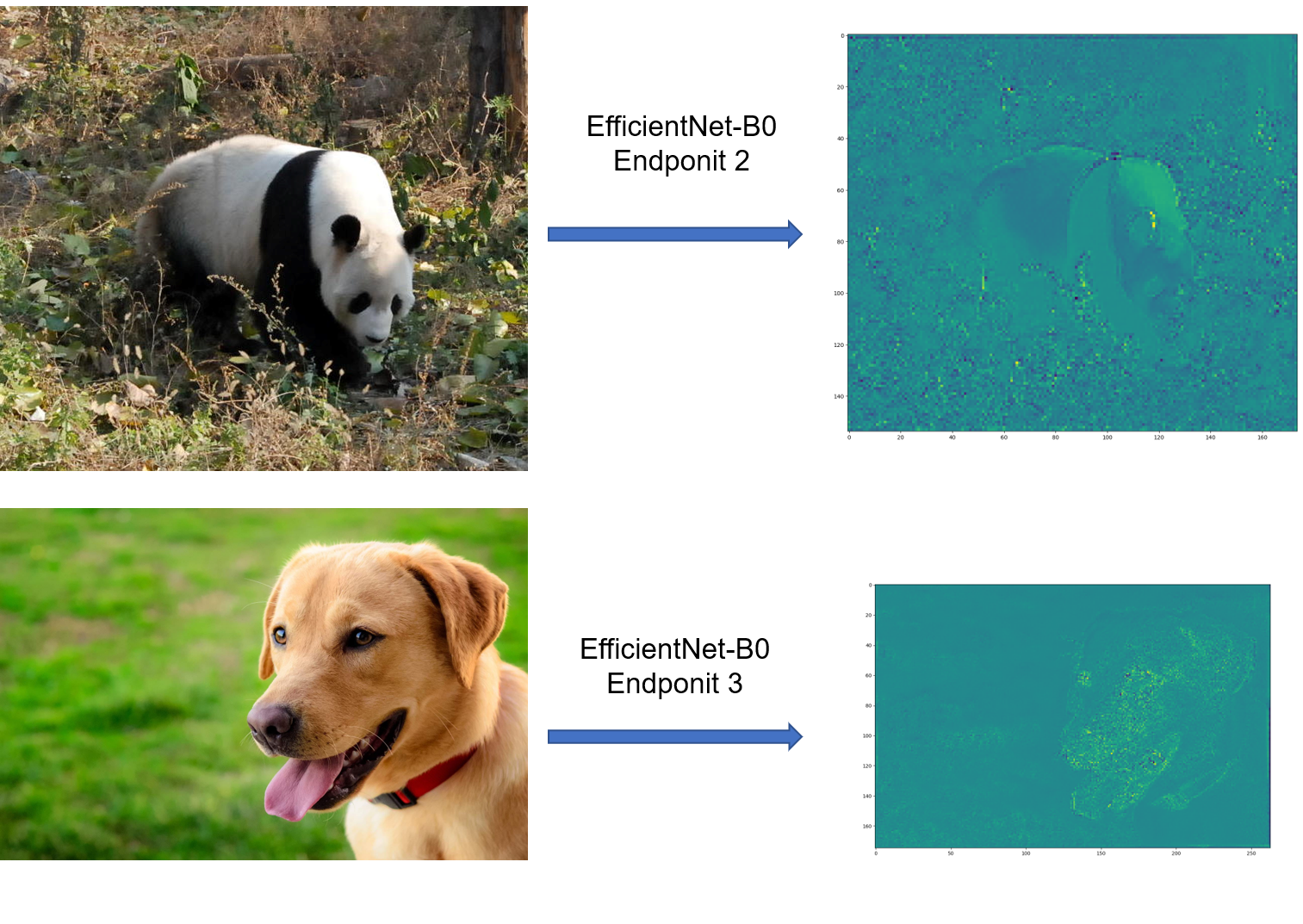
And these endpoints look pretty cool. Totally see the potential for segmentation/detection here.
Activation map (endpoitns) for the panda image and labrador image:
The following code will suffice:
import tensorflow as tf
print(tf.__version__)
import numpy as np
from keras_applications import efficientnet

model = efficientnet.EfficientNetB0(
    include_top=False,
    weights='imagenet',
    input_tensor=None,
    input_shape=(224,224,3),
    pooling=None,
    classes=1,
    backend=tf.keras.backend,
    layers=tf.keras.layers,
    models=tf.keras.models,
    utils=tf.keras.utils
)

model.summary()

model.save('EfficientNet-B0_keras.h5')
Notice that the **kwargs in the function definition are left for the last 4 arguments. I think they can also be set in the init.py file.
Last layer and number of parameters:
top_activation (Activation)     (None, 7, 7, 1280)   0           top_bn[0][0]
==================================================================================================
Total params: 4,049,564
Trainable params: 4,007,548
Non-trainable params: 42,016
__________________________________________________________________________________________________
Appraently we can also leave the image size as (None, None, 3), which does not change the number of parameters at all. It only cares about the channel dimension.
Let's take a look at all the layers and their shape:
block1a_project_bn (?, 112, 112, 16)
block2a_project_bn (?, 56, 56, 24)
block2b_project_bn (?, 56, 56, 24)
block3a_project_bn (?, 28, 28, 40)
block3b_project_bn (?, 28, 28, 40)
block4a_project_bn (?, 14, 14, 80)
block4b_project_bn (?, 14, 14, 80)
block4c_project_bn (?, 14, 14, 80)
block5a_project_bn (?, 14, 14, 112)
block5b_project_bn (?, 14, 14, 112)
block5c_project_bn (?, 14, 14, 112)
block6a_project_bn (?, 7, 7, 192)
block6b_project_bn (?, 7, 7, 192)
block6c_project_bn (?, 7, 7, 192)
block6d_project_bn (?, 7, 7, 192)
block7a_project_bn (?, 7, 7, 320)
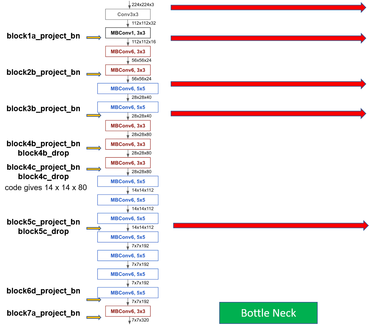
It seems that all the blocks end with batch normalization layers. I think this will be what the U-Net look like after construction:
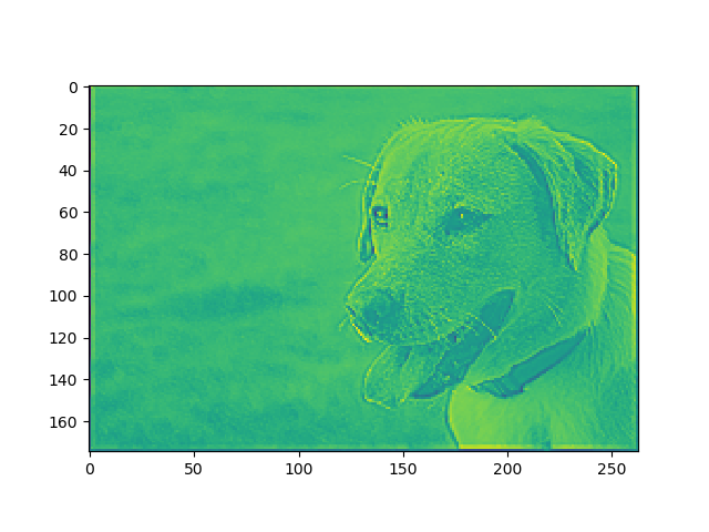
Let's look at the output after block3b_project_bn in the pre-trained network loaded from keras applications:
Code used
input_name = 'labrador'
import imageio
images = imageio.imread("%s.jpg"%input_name)
images = np.reshape(images, (1, images.shape[0], images.shape[1], images.shape[2]))
images = images.astype(np.float32)
print(images.shape, images.dtype)


eunet = efficientnet_unet(input_shape=images.shape[1:])

layer_3b = eunet.get_layer(name='block3b_project_bn')
inter_model = tf.keras.Model(inputs = eunet.input, outputs = layer_3b.output)
activation_maps = inter_model.predict(images)


import matplotlib.pyplot as plt
import os

dev_tmp = r'./../tmp'
ks = [0, 10, 20]
for k in ks:
    plt.imshow(activation_maps[0, :, :, k])
    plt.savefig(os.path.join(dev_tmp, 'keras_3b_channel_%d__%s.png'%(k, input_name)))
    plt.clf()
It's hard to tell whether this proofs that the network is pre-trained or not... Because random weights also give images kind of like this.
-
Bottleneck input: encoder model block7a (not using the top conv layer, which ahas over 1000 filters)
-
First upsampling and concatenation: with encoder model 5c, which is 14 x 14 x 112
-
Second upsampling and concatenation: with encoder model 3b, which is 28 x 28 x 40
-
Third upsampling and concatenation: with encoder model 2b, which is 56 x 56 x 24
-
Fourth upsampling and concatenation: with encoder model 1a (no project bn), which is 112 x 112 x 16
-
Fifth upsampling and concatenation: with encoder model input, which is 224 x 224 x 3, only layer with original shape ( a bit weird, not the same as U-Net)
Check efficientnet_unet/build_eunet.py
So I looked through a few options:
-
- need a organization/school email address just for downloading. So this won't work out.
-
-
tried downloading this using TensorFlow-datasets directly. Won't work because there's some issue unzipping the files. Also, the requirement on disk storage is also crazy
-
Downloading from COCO website directly
-
Figuring out the data format for segmentation (Panoptic?) Maybe use their API pycoco
-
@DONE check out the implementation provided in the keras-applications repo. Seems that this repo has code that's editable in terms of model architecture. Also, it looks much cleaner (?), without too many dependencies. Most of the functions seemed to be implmemented within that same file for efficientnet.
@DONE Add skip connections and everything else to this model. Hopefully we'll get a trainable U-Net soon.
-
basically had a wrapper model, now only need to do skip connections and conv2d and upsampling
-
bottleneck done, did one upsampling and concatenation... I am following the U-Net, with 4 upsampling layers
-
also noticed that the layers should end at "dropout" in the encoder part
@DONE check the efficientnet from Keras with the panda image above, making sure it actually has pre-trained weights
@DONE find some segmentation sets to test the model
@TODO Try ADE20K first, I changed my mind
Checked out this segmentation list from Richard Szeliski's book


