lulcc provides a framework for spatially explicit land use change modelling in r. The long term goal of lulcc is to provide a smart and tidy interface to running the standard land use change modelling in 4 steps: raster data prepping, probability surface generation, allocation and validation, in one tidy package.
You can install the released version of lulcc from CRAN with:
install.packages("lulcc")And the development version from GitHub with:
# install.packages("devtools")
devtools::install_github("simonmoulds/lulcc")Adapted from https://www.geosci-model-dev.net/8/3215/2015/
The package includes two example datasets: one for Sibuyan Island in the Phillipines and one for the Plum Island Ecosystem in Massachusetts, United States. Here we present a complete working example for the Plum Island Ecosystem dataset.
Land use change modelling requires a large amount of input data. The
most important input is at least one map of observed land use. In lulcc,
this data is represented by the ObsLulcRasterStack class:
library(lulcc)
#> Loading required package: raster
#> Loading required package: sp
data(pie)
obs <- ObsLulcRasterStack(x=pie,
                          pattern="lu",
                          categories=c(1,2,3),
                          labels=c("Forest","Built","Other"),
                          t=c(0,6,14))
A useful starting point in land use change modelling is to obtain a
transition matrix for two observed land use maps to identify the main
transitions. This can be achieved with the crossTabulate function:
# obtain a transition matrix from land use maps for 1985 and 1991
crossTabulate(obs, times=c(0,6))
#>        Forest Built Other
#> Forest  46672  1926   415
#> Built       0 37085    37
#> Other     359  1339 25730
For the Plum Island Ecosystem site this reveals that the main transition was from forest to built areas.
The next stage is to relate observed land use or observed land use transitions to spatially explicit biophysical or socioeconomic explanatory variables. These are loaded as follows:
ef <- ExpVarRasterList(x=pie, pattern="ef")To fit predictive models we first divide the study region into training
and testing partitions. The partition function returns a list with
cell numbers for each partition:
part <- partition(x=obs[[1]],
                  size=0.1, spatial=TRUE)
We then extract cell values for the training and testing partitions.
# extract training data
train.data <- getPredictiveModelInputData(obs=obs,
                                          ef=ef,
                                          cells=part[["train"]],
                                          t=0)

test.data <- getPredictiveModelInputData(obs=obs,
                                         ef=ef,
                                         cells=part[["test"]])
Predictive models are represented by the PredictiveModelList class.
For comparison, we create a PredictiveModelList object for each type
of predictive model:
# fit models (note that a predictive model is required for each land use category)
forms <- list(Built~ef_001+ef_002+ef_003,
              Forest~ef_001+ef_002,
              Other~ef_001+ef_002)

# generalized linear model models
glm.models <- glmModels(formula=forms,
                        family=binomial,
                        data=train.data,
                        obs=obs)
#> Warning in if (is.na(categories) | is.na(labels)) {: the condition has length >
#> 1 and only the first element will be used
#> Warning: glm.fit: fitted probabilities numerically 0 or 1 occurred
# recursive partitioning and regression tree models
rpart.models <- rpartModels(formula=forms,
                            data=train.data,
                            obs=obs)
#> Warning in if (is.na(categories) | is.na(labels)) {: the condition has length >
#> 1 and only the first element will be used
# random forest models (WARNING: takes a long time!)
rf.models <- randomForestModels(formula=forms,
                                data=train.data,
                                obs=obs)
#> Warning in if (is.na(categories) | is.na(labels)) {: the condition has length >
#> 1 and only the first element will be used
#> Warning in randomForest.default(m, y, ...): The response has five or fewer
#> unique values. Are you sure you want to do regression?

#> Warning in randomForest.default(m, y, ...): The response has five or fewer
#> unique values. Are you sure you want to do regression?

#> Warning in randomForest.default(m, y, ...): The response has five or fewer
#> unique values. Are you sure you want to do regression?
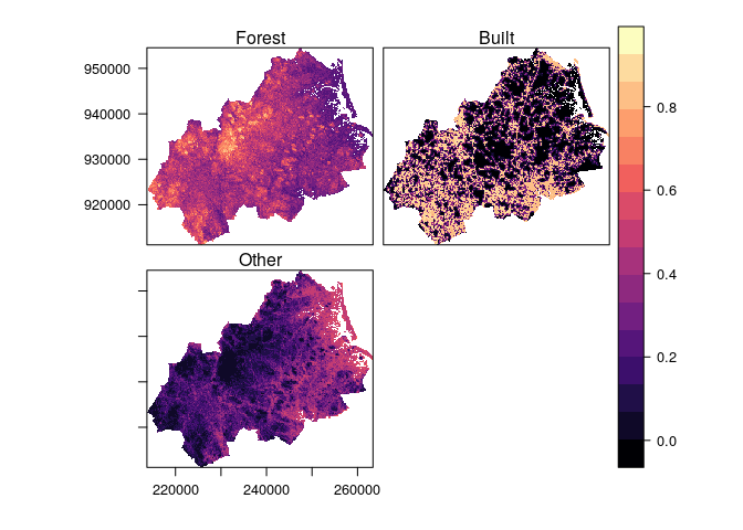
We can then use the fitted models to predict over the full data set and produce the probability surfaces for each fitted model:
all.data <- as.data.frame(x=ef, obs=obs, cells=part[["all"]])

# GLM
probmaps <- predict(object=glm.models,
                    newdata=all.data,
                    data.frame=TRUE)
points <- rasterToPoints(obs[[1]], spatial=TRUE)
probmaps <- SpatialPointsDataFrame(points, probmaps)
probmaps <- rasterize(x=probmaps, y=obs[[1]],
                      field=names(probmaps))
rasterVis::levelplot(probmaps)
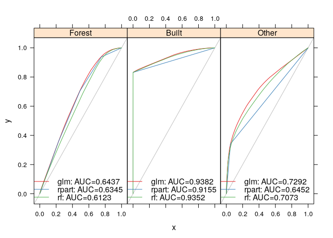
Model performance is assessed using the receiver operator characteristic
provided by the
ROCR package.
lulcc includes classes Prediction and Performance which extend the
native ROCR classes to contain multiple prediction and performance
objects. The procedure to obtain these objects and assess performance is
as follows:
glm.pred <- PredictionList(models=glm.models,
                           newdata=test.data)
glm.perf <- PerformanceList(pred=glm.pred,
                            measure="rch")
rpart.pred <- PredictionList(models=rpart.models,
                             newdata=test.data)
rpart.perf <- PerformanceList(pred=rpart.pred,
                              measure="rch")
rf.pred <- PredictionList(models=rf.models,
                          newdata=test.data)
rf.perf <- PerformanceList(pred=rf.pred,
                           measure="rch")
plot(list(glm=glm.perf,
          rpart=rpart.perf,
          rf=rf.perf))
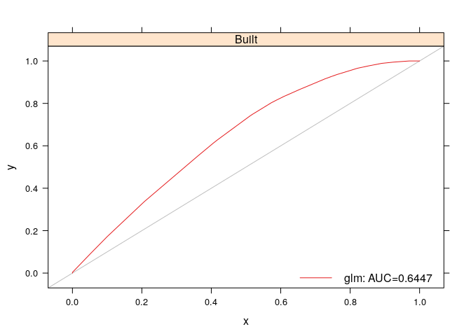
Another use of ROC analysis is to assess how well the models predict the cells in which gain occurs between two time points. This is only possible if a second observed land use map is available for a subsequent time point. Here we perform this type of analysis for the gain of built between 1985 and 1991. First, we create a data partition in which cells not candidate for gain (cells belonging to built in 1985) are eliminated. We then assess the ability of the various predictive models to predict the gain of built in this partition:
part <- rasterToPoints (obs[[1]],
                        fun=function(x) x != 2,
                        spatial=TRUE)
test.data<- getPredictiveModelInputData(obs=obs,
                                        ef=ef,
                                        cells=part,
                                        t=6)
glm.pred <- PredictionList(models=glm.models[[2]],
                           newdata=test.data)
glm.perf <- PerformanceList(pred=glm.pred,
                            measure="rch")
plot(list(glm=glm.perf))Spatially explicit land use change models are usually driven by non-spatial estimates of land use area for each timestep in the simulation. While many complex methods have been devised, in lulcc we simply provide a method for linear extrapolation of land use change, which relies on there being at least two observed land use maps:
# obtain demand scenario
dmd <- approxExtrapDemand(obs=obs, tout=0:14)
#> Warning in total(x = obs): missing argument 'categories': getting categories
#> from 'x'
We then use a filter defined as a matrix within the NeighbRasterStack
function to gather neighbor data from the land use change data.
w <- matrix(data=1, nrow=3, ncol=3)
nb <- NeighbRasterStack(x=obs[[1]], weights=w,
                        categories=c(1,2,3))
The culmination of the modelling process is to simulate the location of land use change. lulcc provides a routine based on the CLUE-S model (Verburg et al., 2002) and a novel stochastic allocation procedure (with option for using the ordered method). The first step is to combine the various model inputs to ensure they are compatible:
clues.rules <- matrix(data=1, nrow=3, ncol=3)
clues.parms <- list(jitter.f=0.0002,
                    scale.f=0.000001,
                    max.iter=1000,
                    max.diff=50,
                    ave.diff=50)
clues.model <- CluesModel(obs=obs,
                          ef=ef,
                          models=glm.models,
                          time=0:14,
                          demand=dmd,
                          elas=c(0.2,0.2,0.2),
                          rules=clues.rules,
                          params=clues.parms)
ordered.model <- OrderedModel(obs=obs,
                              ef=ef,
                              models=glm.models,
                              time=0:14,
                              demand=dmd,
                              order=c(2,1,3))
Then, finally, we can perform allocation:
clues.model <- allocate(clues.model)
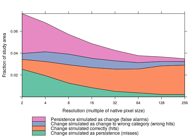
ordered.model <- allocate(ordered.model, stochastic=TRUE)An important yet frequently overlooked aspect of land use change modelling is model validation. lulcc provides a recent validation method developed by Pontius et al. (2011), which simultaneously compares a reference (observed) map for time 1, a reference map for time 2 and a simulated map for time 2. The first step in this method is to calculate three dimensional contingency tables:
# evaluate CLUE-S model output
clues.tabs <- ThreeMapComparison(x=clues.model,
                                   factors=2^(1:8),
                                   timestep=14)
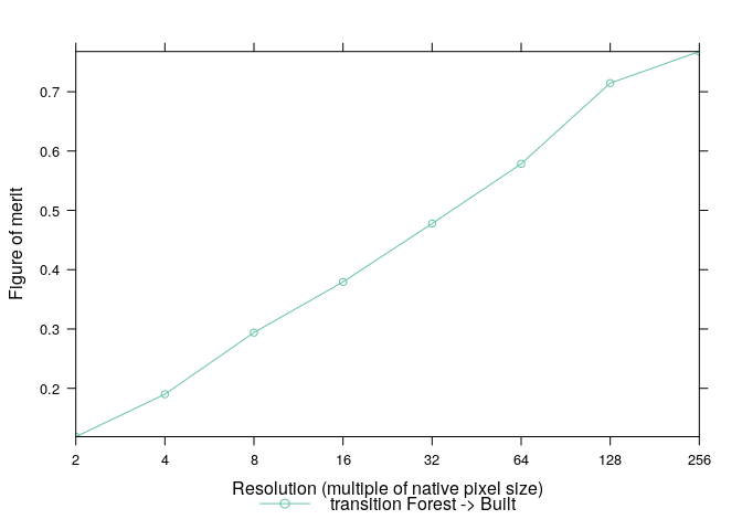
From these tables we can easily extract information about different types of agreement and disagreement as well as compute summary statistics such as the figure of merit:
clues.agr <- AgreementBudget(x=clues.tabs)
plot(clues.agr, from=1, to=2)
clues.fom <- FigureOfMerit(x=clues.agr)
plot(clues.fom, from=1, to=2)