Build a Traffic Sign Recognition Project
The goals / steps of this project are the following:
- Load the data set (see below for links to the project data set)
- Explore, summarize and visualize the data set
- Design, train and test a model architecture
- Use the model to make predictions on new images
- Analyze the softmax probabilities of the new images
- Summarize the results with a written report
Please find below Validation of each rubric points below.
-
Number of training examples = 34799
-
Number of testing examples = 12630
-
Number of validation examples = 4410
-
Image data shape = (32, 32, 3)
-
Number of classes = 43
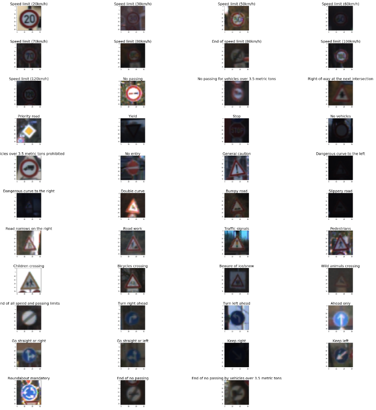
All Sign boards displayed.
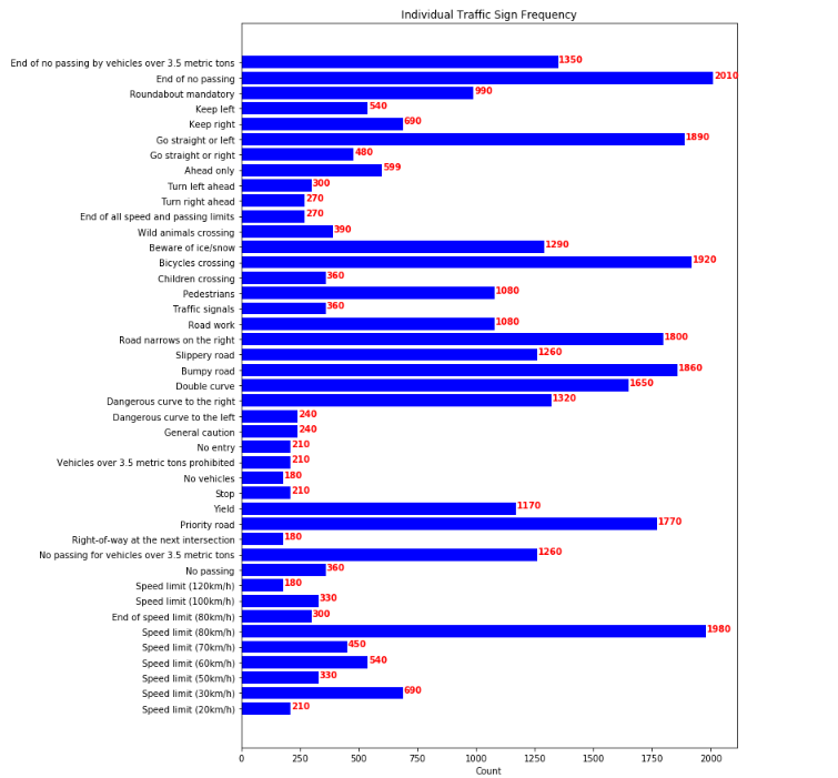
Bar chart showing Frequency of each traffic sign in training set.
Shuffling of dataset using the sklearn.utils library. X_train, y_train = shuffle(X_train, y_train)
Normalizing of images using Adaptive Histogram equalization
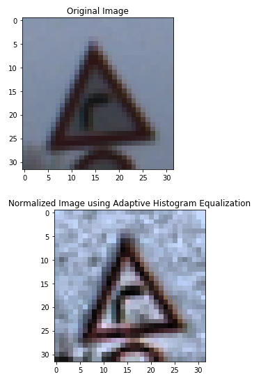
As is apparent from the example above that Histogram equalisation improves the contrast and thus, making it easier for neural network to identify key features fo image during image training
First model was a simple bare bones LeNet architecture.
The problem with the initial architecture were it's inability to generalize. Also, earlier the EPOCHS used were only 10 and the performance starts to plataeu after 20 EPOCHS
First model used did not use the dropout technique. Addition of the technique helped increasing the accuracy and performance on the new images as well.
As mentioned earlier EPOCHS were incresead from 10 to 30 so as to reach the plateau condition with the training
Dropout technique at the last 2 Fully connnected layers, as simple it is to implement, it seems for larger training datasets like ImageNet will perform brilliantly. It increased the genraliszing ability of my network as well.
A good experiment could be to replace Max-pooling with a Convolution layer as dicussed in paper titled Striving for Simplicity: The All Convolutional Net
Modified LeNet for 43 labels
| Layer | Description | Activation Function |
|---|---|---|
| Input | 32x32x3 RGB image | |
| Convolution 1 | 1x1 stride, VALID padding, output = 28x28x6 | RELU |
| Max pooling | 2x2 stride, VALID padding, output = 14x14x6 | |
| Convolution 2 | 1x1 stride, VALID padding, output = 10x10x16 | RELU |
| Max pooling | 2x2 stride, VALID padding, output = 5x5x16 | |
| Flatten | output = 400 | |
| Fully connected 1 with Dropout | input = 400, output = 120 | RELU |
| Fully connected 2 with Dropout | input = 120, output = 84 | RELU |
| Fully connected 3 | input = 84, output = 10 |
epochs = 30
Batch size = 128
learning rate = 0.001.
Training Accuracy(With Validation set created out of training data) = 97 (average) Test Accuracy = 92 (average) Validation Accuracy = 94 (average)
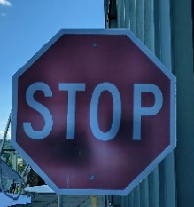
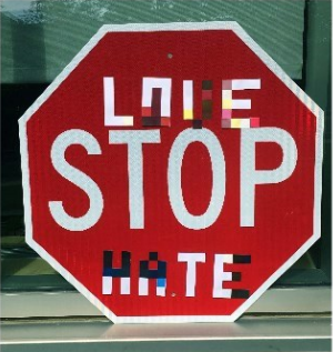
Four Different type of signboards chosen from internet. Two of the images shown below are taken a from a recent paper that says how neural networks can be fooled.
Watching the second image, an added text of 'LOVE HATE' has been added to the stop sign, so while recognising it confuses it with some speed limit sign. This is because of the text, teh neural network doesn't understand the context and hence even if additionally trained to identify English letters, it might fail.
Here is the complete paper for reference: Robust Physical-World Attacks on Machine Learning Models
Here are the results of the prediction:
| Image | Prediction |
|---|---|
| Speed limit (20km/h) | Speed limit (60km/h) |
| Stop | Stop |
| Stop (Noisy) | Speed limit (30km/h) |
| Stop (Noisy) | Speed limit (30km/h) |
| Stop(With Background) | Stop |
| No entry | No entry |
| Speed limit (70km/h) | Speed limit (60km/h) |
The model was able to correctly predict 5 other 7 traffic signs, which gives an accuracy of 71% comapring it with the images provided in with test dataset(92%) it is really low. Mostly beacuse of the 2 tricky images out of 7 that were used.
3. Describe how certain the model is when predicting on each of the five new images by looking at the softmax probabilities for each prediction. Provide the top 5 softmax probabilities for each image along with the sign type of each probability.
All the Softmax probabilities have been plotted alongside images. The top5 softmax probabilities for new images is shown below:
i1_0.png: Correct Answer : Speed limit (20km/h)
Speed limit (60km/h): 93.55%
Speed limit (30km/h): 6.45%
Speed limit (80km/h): 0.00%
Speed limit (70km/h): 0.00%
Traffic signals: 0.00%
i4a_14.png: Correct Answer : Stop
Stop: 99.99%
Speed limit (60km/h): 0.01%
Speed limit (80km/h): 0.00%
Speed limit (20km/h): 0.00%
Speed limit (30km/h): 0.00%
i1_17.png: Correct Answer : No entry
No entry: 100.00%
No vehicles: 0.00%
Stop: 0.00%
Speed limit (30km/h): 0.00%
Turn right ahead: 0.00%
i4c_14.png: Correct Answer : Stop
Speed limit (30km/h): 88.00%
Speed limit (70km/h): 6.36%
Speed limit (60km/h): 2.54%
Speed limit (80km/h): 2.14%
Stop: 0.94%
i4d_14.png: Correct Answer : Stop
Speed limit (30km/h): 53.35%
Stop: 46.63%
General caution: 0.02%
Traffic signals: 0.00%
Speed limit (60km/h): 0.00%
i4b_14.png: Correct Answer : Stop
Stop: 100.00%
Speed limit (30km/h): 0.00%
Speed limit (50km/h): 0.00%
Speed limit (70km/h): 0.00%
Yield: 0.00%
i3_4.png: Correct Answer : Speed limit (70km/h)
Speed limit (60km/h): 75.45%
Speed limit (30km/h): 14.57%
Speed limit (70km/h): 9.87%
Speed limit (80km/h): 0.07%
General caution: 0.03%%

