This project was created as an assessment for the Self-Driving Car Nanodegree Program by Udacity. The goal is to detect lane lines on videos, calculate the curvature of the lane and the offset of the car from the center.
Click on the image to play the video.
| Track 1 | Track 1 + Debugging |
|---|---|
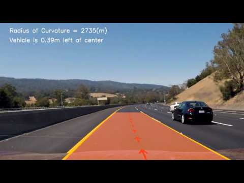 |
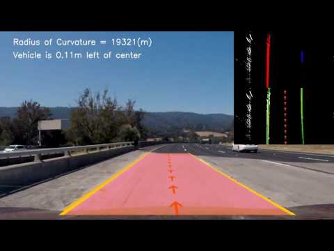 |
| Track 2 | Track 2 + Debugging |
|---|---|
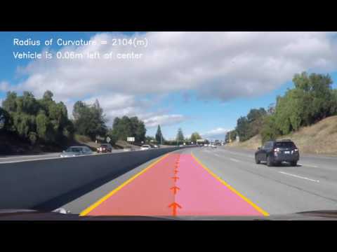 |
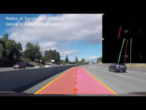 |
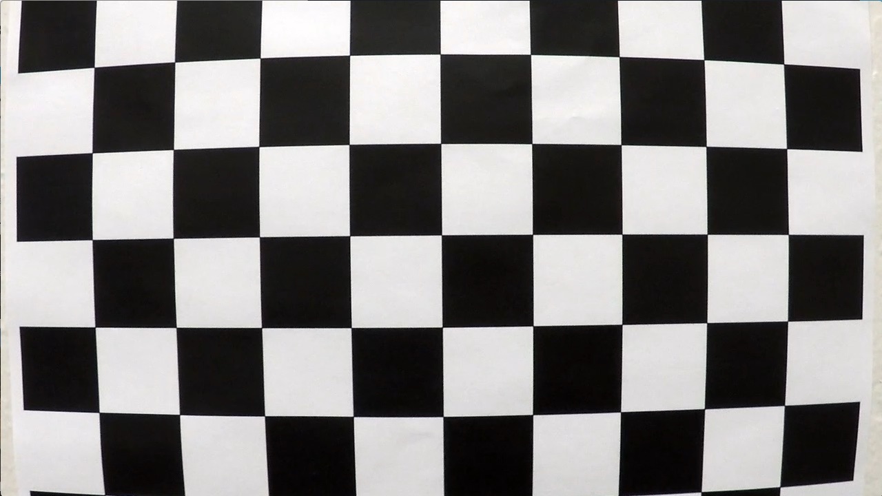
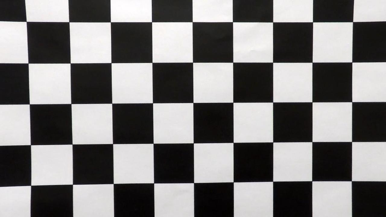
Images or videos captured by a camera are typically distorted by the lens. Using a image like that would cause problems when trying to calculate the curvature or the car's offset to the center line. That's why it is important to undistort images first. For that a distortion matrix is calculated based on several images of a chessboard captured by the same camera. The matrix can then be used to undistort other images.
| Original | Undistorted |
|---|---|
 |
 |
In the following section, the different steps of the lane detection pipeline are described in the same order as they are apply in the algorithm.
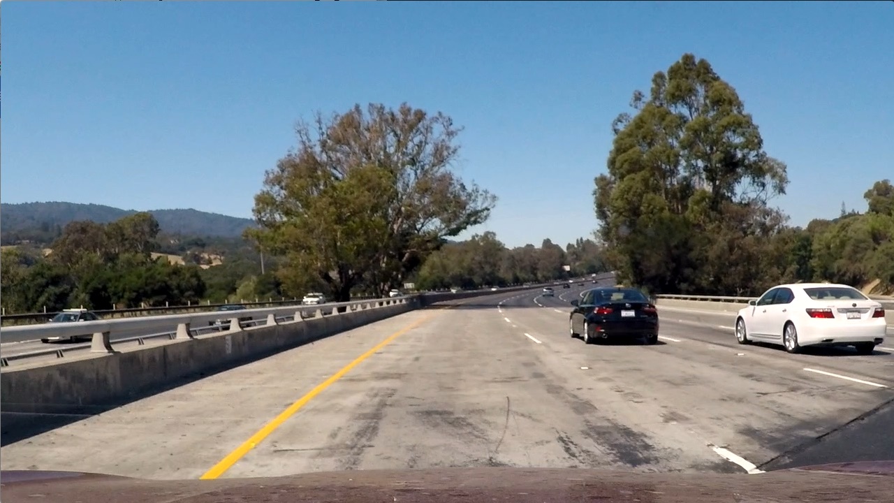
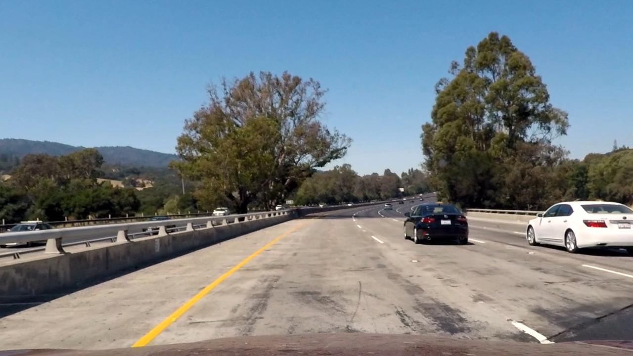
The first step is to remove the lens distortion by applying the calculated distortion matrix.
| Original | Undistorted |
|---|---|
 |
 |
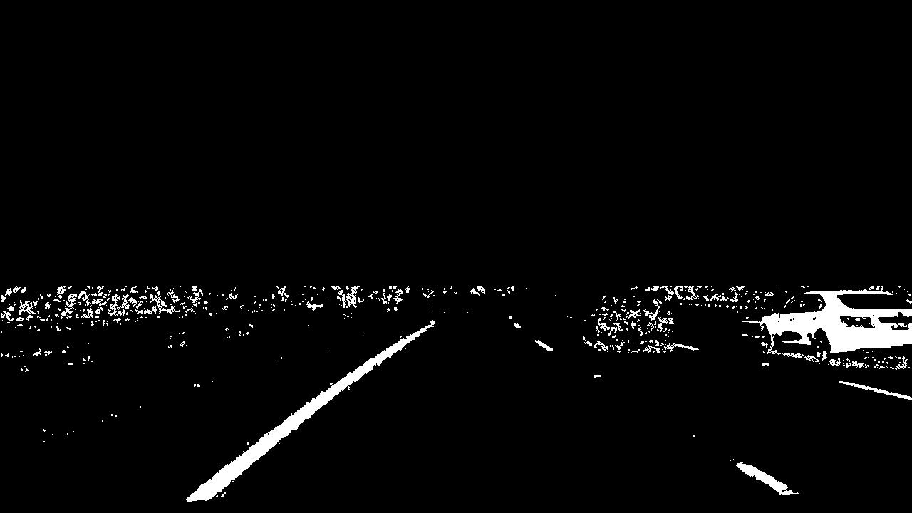
After the lens distortion has been removed, a binary image will be created, containing pixels which are likely part of a
lane. Therefore the result of multiple techniques are combined by a bitwise and operator. Finding good parameters for the different techniques like threshold values is quite challenging. To improve the feedback cycle of applying different parameters, an interactive [jupyter notebook](Interactive Parameter Exploration.ipynb) was created.
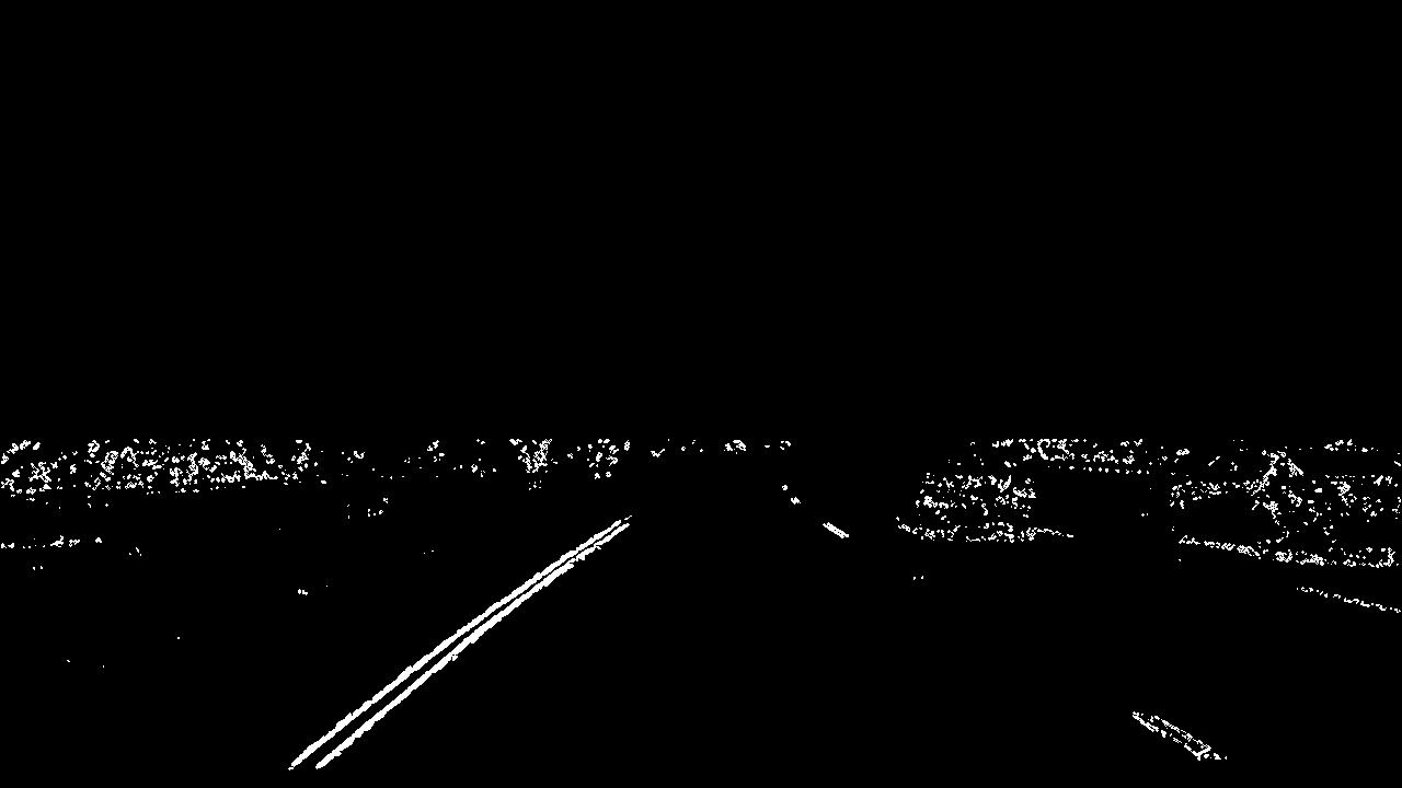
The first technique is called sobel operation which is able to detect edges by computing an approximation of the
gradient of the image intensity function. The operation was applied for both directions (x and y) and combined to keep only
those pixel which are on both results and also over a specified threshold. An averaged gray scale image from
the U and V color channels of the YUV space and also the S channel of the HLS space was used as input.
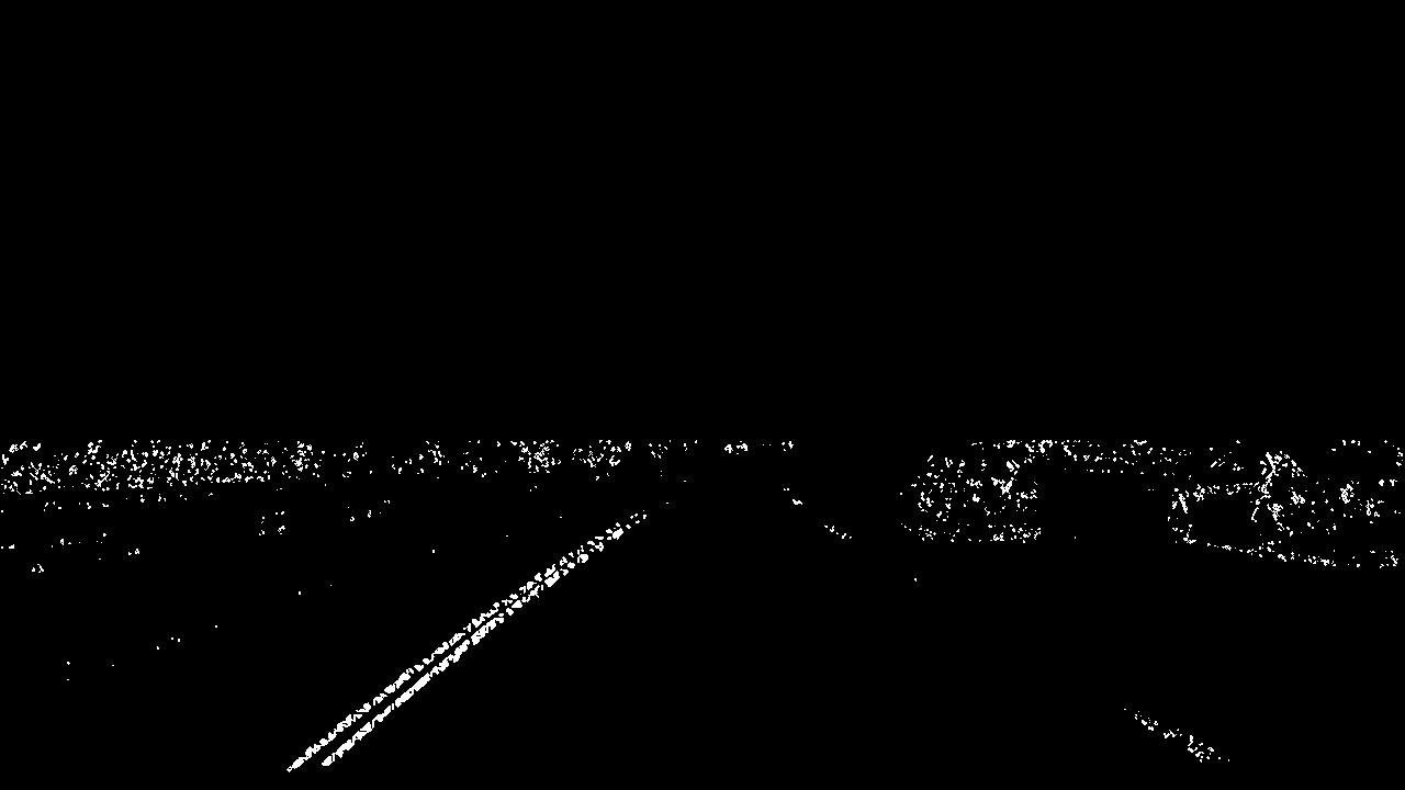
Additionally, the magnitude and direction of the gradient was calculated and combined by keeping only pixels with values above a threshold (different threshold for magnitude and direction) on both images.
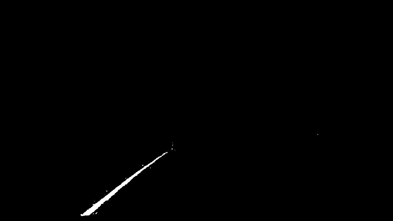
Technique number three is a basic color thresholding which tries to isolate yellow pixels.
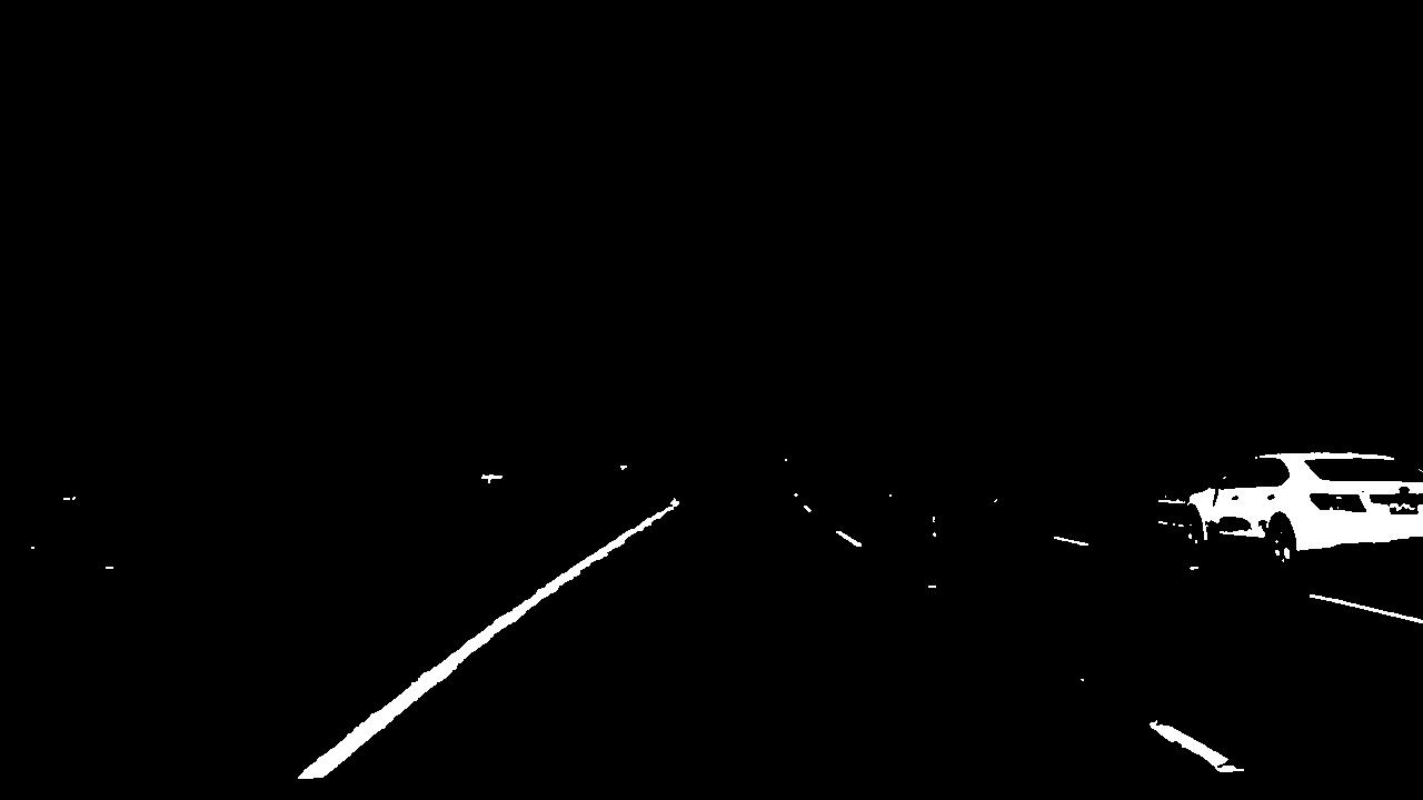
The last technique is an adaptive highlight / high intensity detection. It isolates all the pixels which have values above
a given percentile in order to make it more resilient against different lighting conditions.
In the end, the results are combined through a bitwise or operation to get the final lane mask.
| Sobel X & Y | Magnitude & Direction of Gradient | Yellow | Highlights | Combined |
|---|---|---|---|---|
 |
 |
 |
 |
 |
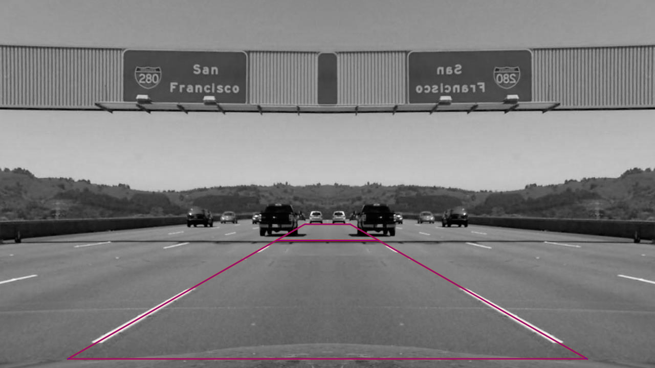
To determine suitable source coordinates for the perspective transformation, an image with relative straight lines was used as reference. Since the car was not perfectly centered the image, it was horizontally mirrored. The resulting image was then used inside the interactive [jupyter notebook](Interactive Parameter Exploration.ipynb) to fit vanishing lines and to get source coordinates.
| Reference | Transformed |
|---|---|
 |
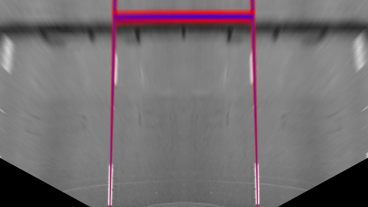 |
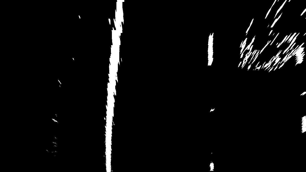
After suitable coordinates were determined, the transformation can be applied to other images. This is of course just an approximation and is not 100% accurate.
| Mask | Birdseye View |
|---|---|
 |
 |
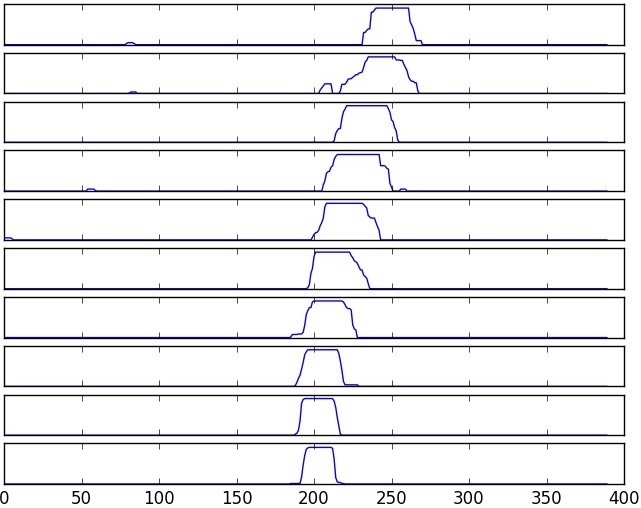
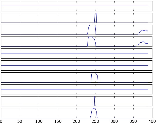
Since not all pixels marked in the mask are actually part of the lanes, the most likely ones have to be identified. For that, a sliding histogram is applied to detect clusters of marked pixels. The highest peak of each histogram is used as the center of a window which assigns each pixel inside to the corresponding lane. The sliding histogram is applied to the left half of the image to detect left line pixels and applied on the right half of the image to detect right lane pixels. Therefore, the algorithm will fail if a lane crosses the center of the image.
This process is pretty computing intensive. That's why the algorithm will try to find lane pixels in the area of
previously found lines first. This is only possible when using videos.
| Left Lane Histogram | Assigned Pixels | Right Lane Histogram |
|---|---|---|
 |
 |
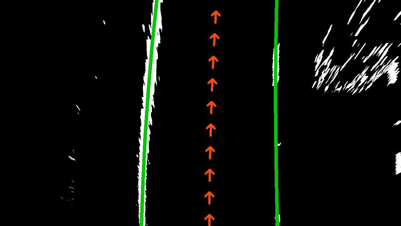
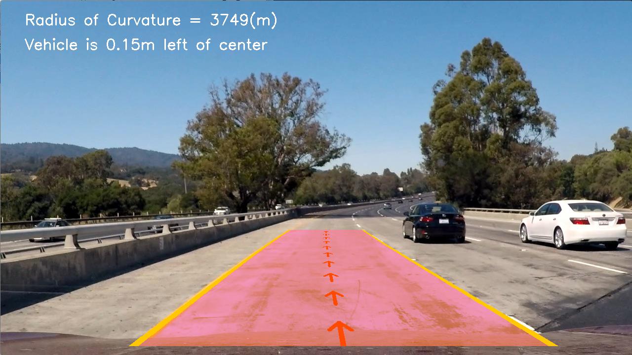
With pixels assigned to each lane, a second order polynomials can be fitted. To achieve smoother results, the polynomials are also average over the last five frames in a video. The polynomials are also used to calculate the curvature of the lane and the relative offset from the car to the center line.
| Fit Polynomial | Final |
|---|---|
 |
 |
