Algorithm Collab

AASAAM Algorithm & Data Structures Collaboration notes and codes

What is the goal of this collaboration?

The goal of this collaboration is to learn and practice algorithms and data structures together. We will be using Python and JavaScript as our main programming language.

Why Algorithms and Data Structures?

Algorithms and data structures are the backbone of computer science and software development. Understanding these topics is crucial because they form the foundation for efficient problem-solving, enabling us to create better, faster, and more scalable software.

Time Complexity

Time complexity is a measure of how the running time of an algorithm increases with the size of the input data.

Big O Notation (O-notation):
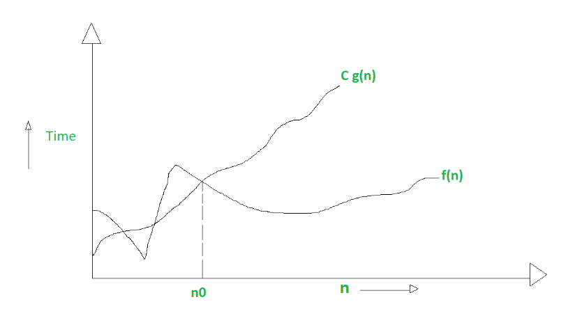
- Formal Definition: The time complexity of an algorithm is said to be O(g(n)) if there exist positive constants C and n₀ such that for all values of n greater than or equal to n₀, the running time of the algorithm is at most C times the growth rate of the function g(n).
- Graphical Representation:
- Mathematical Definition:
```
f(n) is in O(g(n)) if there exist positive constants C and n₀ such that for all values of n ≥ n₀:
0 ≤ f(n) ≤ C * g(n)
```
Big Omega Notation (Ω-notation):
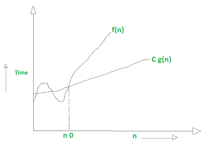
- Formal Definition: The time complexity of an algorithm is said to be Ω(g(n)) if there exist positive constants C and n₀ such that for all values of n greater than or equal to n₀, the running time of the algorithm is at least C times the growth rate of the function g(n).
- Graphical Representation:
- Mathematical Definition:
```
f(n) is in Ω(g(n)) if there exist positive constants C and n₀ such that for all values of n ≥ n₀:
0 ≤ C * g(n) ≤ f(n)
```
Big Theta Notation (Θ-notation):
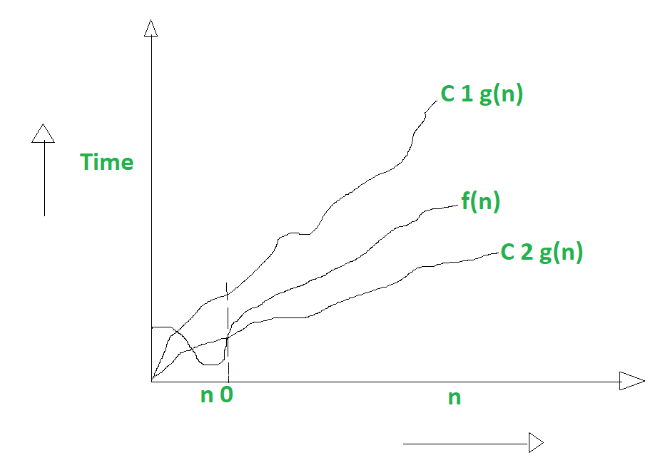
- Formal Definition: The time complexity of an algorithm is said to be Θ(g(n)) if there exist positive constants C₁, C₂, and n₀ such that for all values of n greater than or equal to n₀, the running time of the algorithm is at least C₁ times the growth rate of the function g(n) and at most C₂ times the growth rate of the function g(n).
- Graphical Representation:
- Mathematical Definition:
```
f(n) is in Θ(g(n)) if there exist positive constants C₁, C₂, and n₀ such that for all values of n ≥ n₀:
0 ≤ C₁ * g(n) ≤ f(n) ≤ C₂ * g(n)
```

Some Common Time Complexities

Notation	Name	Example
O(1)	Constant	Accessing a specific element in an array by index
O(log n)	Logarithmic	Finding an element in a sorted array with a binary search
O(n)	Linear	Finding an element in an unsorted array with a linear search
O(n log n)	Log-linear	Sorting an array with merge sort or quick sort
O(n²)	Quadratic	Finding all possible pairs in an array with a nested loop
O(n³)	Cubic	Finding all possible triplets in an array with a triple nested loop
O(2ⁿ)	Exponential	Finding all subsets of a set with a power set algorithm
O(n!)	Factorial	Finding all permutations of a string or array with a permutation algorithm
O(nⁿ)	Polynomial	Finding all possible paths in a graph with a brute-force algorithm

Examples

Constant Time Complexity (O(1)):

def constant_time_complexity(arr):
    return arr[0]

Linear Time Complexity (O(n)):

def linear_time_complexity(arr):
    for i in arr:
        print(i)

Quadratic Time Complexity (O(n²)):

def quadratic_time_complexity(arr):
    for i in arr:
        for j in arr:
            print(i, j)

Cubic Time Complexity (O(n³)):

def cubic_time_complexity(arr):
    for i in arr:
        for j in arr:
            for k in arr:
                print(i, j, k)

Logarithmic Time Complexity (O(log n)):

def logarithmic_time_complexity(arr):
    i = len(arr)
    while i > 0:
        print(arr[i])
        i = i // 2

Log-Linear Time Complexity (O(n log n)):

def log_linear_time_complexity(arr):
    for i in arr:
        j = len(arr)
        while j > 0:
            print(i, arr[j])
            j = j // 2

Exponential Time Complexity (O(2ⁿ)):

def exponential_time_complexity(n):
    if n <= 0:
        return 1
    return exponential_time_complexity(n - 1) + exponential_time_complexity(n - 1)

Factorial Time Complexity (O(n!)):

def factorial_time_complexity(n):
    if n <= 0:
        return 1
    return n * factorial_time_complexity(n - 1)

Polynomial Time Complexity (O(nⁿ)):

def polynomial_time_complexity(n):
    if n <= 0:
        return 1
    return n * polynomial_time_complexity(n)

Exercises

These are some rough exercises that you use everyday in your codes. Try to find the time complexity of each one of them. some of them are really hard to find the exact time complexity, so you can just give a rough estimation.

def foo(n):
    i = 1
    while i < n:
        print(i)
        i = i * 2

Hint: give attention to the while loop condition and the value of i in each iteration.

:
```
def foo(n):
    i = 1
    while i < n:
        j = 1
        while j < n:
            print(i, j)
            j = j * 3
        i = i * 2
```
Hint: give attention to the while loop condition and the value of i and j in each iteration. Some people might think that the time complexity of this function is O(n²), but it's not. It's actually SOME THING THAT YOU ARE GONNA FIND OUT.

Space Complexity

Space complexity is a measure of how much auxiliary memory an algorithm needs.

Example:

def foo(n):
    arr = []
    for i in range(n):
        arr.append(i)
    return arr

In this example, we are creating an array with n elements. So the space complexity of this function is O(n).

But, with a little improvement:

def foo(n):
    return [i for i in range(n)]

We have still the same Time Complexity: O(n) but, the Space Complexity is O(1).

Exercise

Improve 9th Example above

Divide and Conquer

The divide and conquer algorithm is a method of solving a problem by breaking it down into smaller sub-problems, solving each of those sub-problems once, and then combining them to get the final solution.

Pros

It's a very efficient way to solve a large problem.
Parallelism and Multi-Threading is possible.
Optimal substructure.
Ease of Implementation.

Cons

It's not efficient for small problems.
Recursion overhead.
Memory consumption.
Debugging is difficult.
Not Always Optimal.

Examples

Some of the most famous algorithms that use the divide and conquer technique are:

Merge Sort.
Multiplication of two large numbers.

Quick Sort

The Quick Sort algorithm is a divide and conquer algorithm. It works by selecting a 'pivot' element from the array and partitioning the other elements into two sub-arrays, according to whether they are less than or greater than the pivot. The sub-arrays are then sorted recursively. This can be done in-place, requiring small additional amounts of memory to perform the sorting.

smrrazavian/algorithm_collab

Algorithm Collab

What is the goal of this collaboration?

Why Algorithms and Data Structures?

Time Complexity

Some Common Time Complexities

Examples

Exercises

Space Complexity

Exercise

Divide and Conquer

Pros

Cons

Examples

Quick Sort

Data Structures

Array

Linked List

Stack

Queue

Hash Table

Tree

Heap

Algorithms

Sorting

Searching

Graph

Greedy

Dynamic Programming

Recursion

Divide and Conquer

Backtracking

BFS

DFS