migraph 


About the package
The most commonly used R packages available for network analysis, such
as {igraph} or {sna}, are mainly oriented around directed or
undirected one-mode networks. But researchers are increasingly
interested in analysing multimodal (one-, two-, or three-mode),
multilevel (connected multimodal networks), or multilayer (multiplex or
signed) networks. Existing procedures typically involve ‘projecting’
them into one-mode networks so that they can be used with those tools,
but thereby potentially losing important structural information, or
require one or more other specific packages. Translating between
packages various syntaxes and expectations can introduce significant
transaction costs though, driving confusion, inefficiencies, and errors.
{migraph} builds upon {manynet} to offer smart solutions to these
problems. It includes functions for marking and measuring networks and
their nodes and ties, identifying motifs and memberships in them, and
modelling these networks or simulating processes such as diffusion upon
them. Based on {manynet}, every function works for any compatible
network format - from base R matrices or edgelists as data frames,
{igraph}, {network},
or {tidygraph}
objects. This means it is compatible with your existing workflow, is
extensible by other packages, and uses the most efficient algorithm
available for each task.
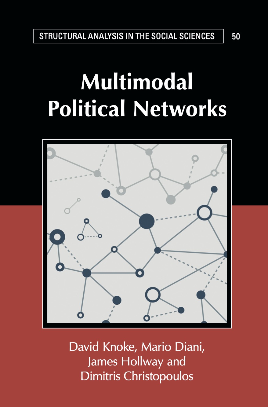
The package is intended as a software companion to the book:
David Knoke, Mario Diani, James Hollway, and Dimitris Christopoulos (2021) Multimodal Political Networks. Cambridge University Press: Cambridge.
Most datasets used in the book are included in this package, and the package implements most methods discussed in the book. Since many of theses datasets and routines are discussed and analysed more there, if you like the package please check out the book, and vice versa.
How does migraph help?
{migraph} includes five special groups of functions, each with their
own pretty print() and plot() methods: marks, measures, memberships,
motifs, and models.
{migraph} uses a common syntax to help new and experienced network
analysts find the right function and use it correctly. All network_*()
functions return a value for the network/graph or for each mode in the
network. All node_*() functions return values for each node or vertex
in the network. And all tie_*() functions return values for each tie
or edge in the network. Functions are given intuitive and succinct names
that avoid conflicts with existing function names wherever possible. All
results are normalised by default, facilitating comparison.
Marks and Measures
{migraph}’s *is_*() functions offer fast logical tests of various
properties. Whereas is_*() returns a single logical value for the
network, node_is_*() returns a logical vector the length of the number
of nodes in the network, and tie_is_*() returns a logical vector the
length of the number of ties in the network.
is_acyclic(),is_aperiodic(),is_bipartite(),is_connected(),is_eulerian(),is_perfect_matching()node_is_core(),node_is_cutpoint(),node_is_isolate(),node_is_max(),node_is_min(),node_is_random()tie_is_bridge(),tie_is_loop(),tie_is_max(),tie_is_min(),tie_is_multiple(),tie_is_reciprocated()
The *is_max() and *is_min() functions are used to identify the
maximum or minimum, respectively, node or tie according to some measure
(see below).
{migraph} also offers a large and growing smorgasbord of measures that
can be used at the node, tie, and network level. Each recognises whether
the network is directed or undirected, weighted or unweighted, one-mode
or two-mode. All return normalized values wherever possible, though this
can be overrided. Here are some examples:
- Centrality:
node_degree(),node_closeness(),node_betweenness(), andnode_eigenvector() - Centralization:
network_degree(),network_closeness(),network_betweenness(), andnetwork_eigenvector() - Cohesion:
network_density(),network_reciprocity(),network_transitivity(),network_equivalency(), andnetwork_congruency() - Connectedness:
network_components(),network_cohesion(),network_adhesion(),network_diameter(),network_length() - Diversity:
network_diversity(),network_homophily(),network_assortativity(),node_diversity(),node_homophily(),node_assortativity(),node_richness() - Innovation: e.g.
node_redundancy(),node_effsize(),node_efficiency(),node_constraint(),node_hierarchy() - Topological features: e.g.
network_core(),network_factions(),network_modularity(),network_smallworld(),network_balance()
Please explore the list of functions to find out more.
Motifs and Memberships
The package also include functions for returning various censuses at the network or node level, e.g.:
network_brokerage_census(),network_dyad_census(),network_mixed_census(),network_triad_census()node_brokerage_census(),node_path_census(),node_quad_census(),node_tie_census(),node_triad_census()
These can be analysed alone, or used as a profile for establishing
equivalence. {migraph} offers both HCA and CONCOR algorithms, as well
as elbow, silhouette, and strict methods for k-cluster selection.
node_automorphic_equivalence(),node_equivalence(),node_regular_equivalence(),node_structural_equivalence()
{migraph} also includes functions for establishing membership on other
bases, such as typical community detection algorithms, as well as
component and core-periphery partitioning algorithms.
Models
All measures can be tested against conditional uniform graph (CUG) or quadratic assignment procedure (QAP) distributions using:
test_permutation(),test_random()
Hypotheses can also be tested within multivariate models via multiple (linear or logistic) regression QAP:
network_reg()
{migraph} is the only package that offers these testing frameworks for
two-mode networks as well as one-mode networks.
Lastly, {migraph} also includes functions for simulating diffusion or
learning processes over a given network:
play_diffusion(),play_diffusions(),play_learning(),play_segregation()
The diffusion models include not only SI and threshold models, but also SIS, SIR, SIRS, SIER, and SIERS.
Installation
Stable
The easiest way to install the latest stable version of {migraph} is
via CRAN. Simply open the R console and enter:
install.packages('migraph')
You can then begin to use {migraph} by loading the package:
library(migraph)
This will load any required packages and make the data contained within the package available. The version from CRAN also has all the vignettes built and included. You can check them out with:
vignettes(package = "migraph")
Development
For the latest development version, for slightly earlier access to new features or for testing, you may wish to download and install the binaries from Github or install from source locally.
The latest binary releases for all major OSes – Windows, Mac, and Linux – can be found here. Download the appropriate binary for your operating system, and install using an adapted version of the following commands:
- For Windows:
install.packages("~/Downloads/migraph_winOS.zip", repos = NULL) - For Mac:
install.packages("~/Downloads/migraph_macOS.tgz", repos = NULL) - For Unix:
install.packages("~/Downloads/migraph_linuxOS.tar.gz", repos = NULL)
To install from source the latest main version of {migraph} from
Github, please install the {remotes} or {devtools} package from CRAN
and then:
- For latest stable version:
remotes::install_github("snlab-ch/migraph", build_vignettes = TRUE) - For latest development version:
remotes::install_github("snlab-ch/migraph@develop", build_vignettes = TRUE)
Tutorials
This package has recently moved away from the use of vignettes, in
favour of smaller and more interactive {learnr} tutorials. Since
version 0.12.3, many of the previous vignettes are instead available as
tutorials, more will be converted soon, and those that have been
converted will continue to be updated and enriched.
To access the tutorials, you will need to have the additional package
{learnr} installed: install.packages("learnr"). Then we would first
suggest that you check to see which vignettes are currently available:
learnr::available_tutorials("migraph")
#> Available tutorials:
#> * migraph
#>   - tutorial3 : "Centrality"
#>   - tutorial4 : "Community"
#>   - tutorial5 : "Equivalence"
#>   - tutorial6 : "Topology"
#>   - tutorial7 : "Diffusion"
#>   - tutorial8 : "Regression"
You can then choose to begin a tutorial using the following command:
e.g. learnr::run_tutorial("tutorial3", "migraph"). For more details on
the {learnr} package, see here.
Relationship to other packages
It draws together, updates, and builds upon many functions currently
available in other excellent R packages such as
{bipartite},
{multinet},
{tnet}, and
{xUCINET}.
Funding details
Most work on this package has been funded by the Swiss National Science Foundation (SNSF) Grant Number 188976: “Power and Networks and the Rate of Change in Institutional Complexes” (PANARCHIC).