CarND-Advanced-Lane-Lines: A Jupyter Notebook repository from solix

Writeup Soheil jahanshahi P4

Advanced Lane Finding Project

The goals / steps of this project are the following:

Compute the camera calibration matrix and distortion coefficients given a set of chessboard images.
Apply a distortion correction to raw images.
Use color transforms, gradients, etc., to create a thresholded binary image.
Apply a perspective transform to rectify binary image ("birds-eye view").
Detect lane pixels and fit to find the lane boundary.
Determine the curvature of the lane and vehicle position with respect to centre.
Warp the detected lane boundaries back onto the original image.
Output visual display of the lane boundaries and numerical estimation of lane curvature and vehicle position.

The project consist of following files:

camera_calib.py: calibrating images using 6 * 9 corner chess boards and saving it to a pickle file
camera_calib/calib_dist_mtx.p: saved pickle file for distortion coefficients and calibration matrix
pipeline.py: pipeline to process images will draw detected line on original image
helper.py : helper functions to use during pipeline
Line.py : line tracker for recent best line, used for robust drawing on the video
video_gen.py : generate a video result for detected lane lines in a video
tracked_video.mp4 : result of lane detection in a video

Writeup / README

Camera Calibration

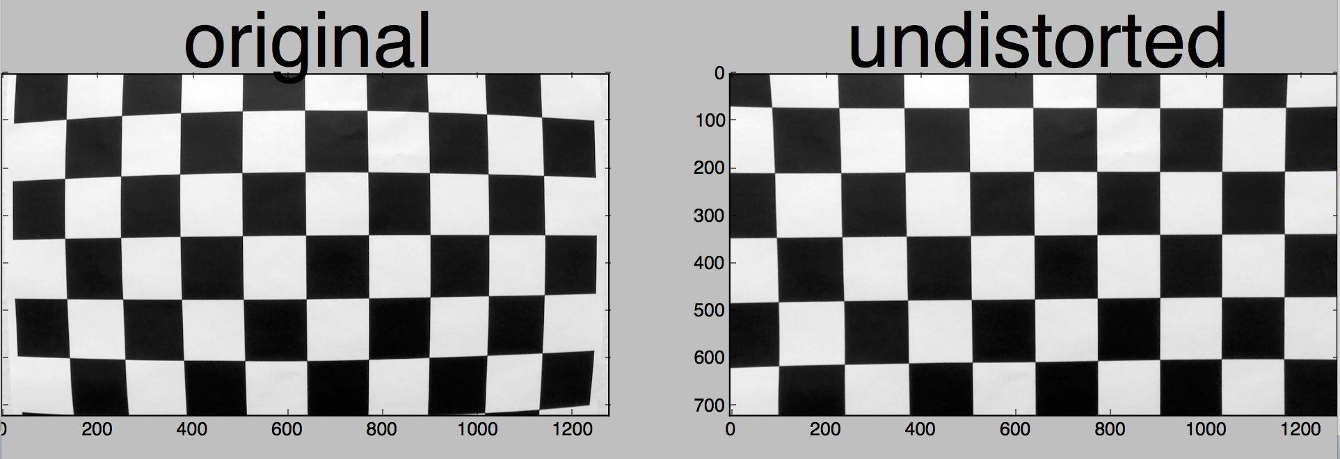
1. Briefly state how you computed the camera matrix and distortion coefficients. Provide an example of a distortion corrected calibration image.

The code for this step is contained in the file called camera_calib.py

I start by preparing "object points", which will be the standard points in the world, we will fill a 2d array for x=6 and y=9 so that means we populate points from (0,0,0) .....(8,5,0) in objp object. For finding image points Opencv function cv2.findChessboardCorners() is used. this will return corners/image points. I then append each objp and corners to the img_points and obj_points list.

I then used the output obj_points and img_points to compute the camera calibration and distortion coefficients using the cv2.calibrateCamera() function. I applied this distortion correction to the test image using the cv2.undistort() function and obtained this result:

in the end I dumped calculated values to a pickle file.

Pipeline (single images)

1. Provide an example of a distortion-corrected image.

To demonstrate this step, I will describe how I apply the distortion correction to one of the test images like this one: 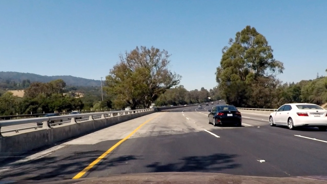you can find the function cal_undistort(img, mtx, dist) in helper.py

First I load the pickle file to extract matrix corners and distortion coefficients and then I use cv2.undistort function to un-distort images, for mtx and dist I should pass the data from pickle file loaded earlier because that has the right values for calibration.

2. Describe how (and identify where in your code) you used color transforms, gradients or other methods to create a thresholded binary image. Provide an example of a binary image result.

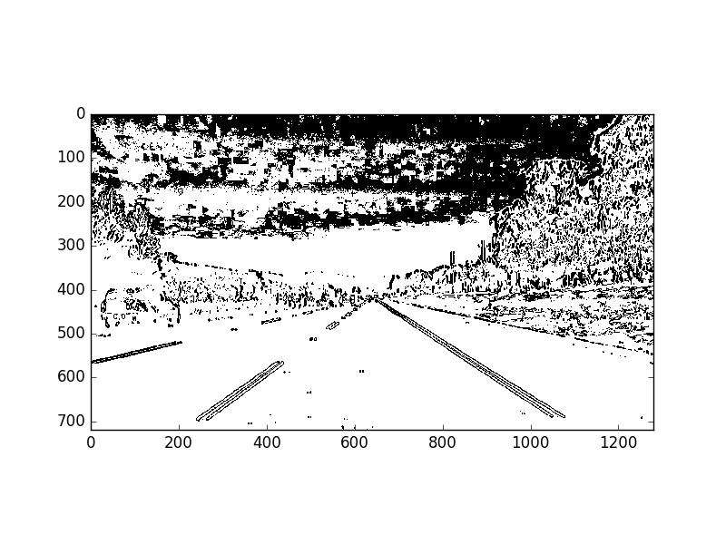
I used a combination of saturate channel color(S in HLS) and gradient in X direction (using cv2.Sobel function) to generate a binary image (thresholding steps at 35 to 37 in pipeline.py). Sobel X operator with kernel size ksize = 15 has shown robust result to extract parallel lines cleanly with thresholding ratio between min = 15 and max = 100. Moreover I combine X gradient image with thresholded S channel. For S channel I used threshold between min=90 and max=255. It was a lot of experimenting!

Here's an example of my output for this step.

3. Describe how (and identify where in your code) you performed a perspective transform and provide an example of a transformed image.

The code for my perspective transform includes a function called warp(), which appears in lines 59 through 67 in the file helper.py . The warp() function takes as inputs an image (img), as well as source (src) and destination (dst) points. I chose the hardcode the source and destination points in the following manner:

src = np.float32([[270, 700], [540, 500], [1220, 700], [800, 500]])
dst = np.float32([[270, 700], [270, 500], [1180, 700], [1180, 500]])

This resulted in the following source and destination points:

Source	Destination
270, 700	270, 700
540, 500	270, 500
1220, 700	1180, 700
800, 500	1180, 500

Pipeline for waring image: I started out by drawing four source points on image; two for each vertical line of a lane, like this:

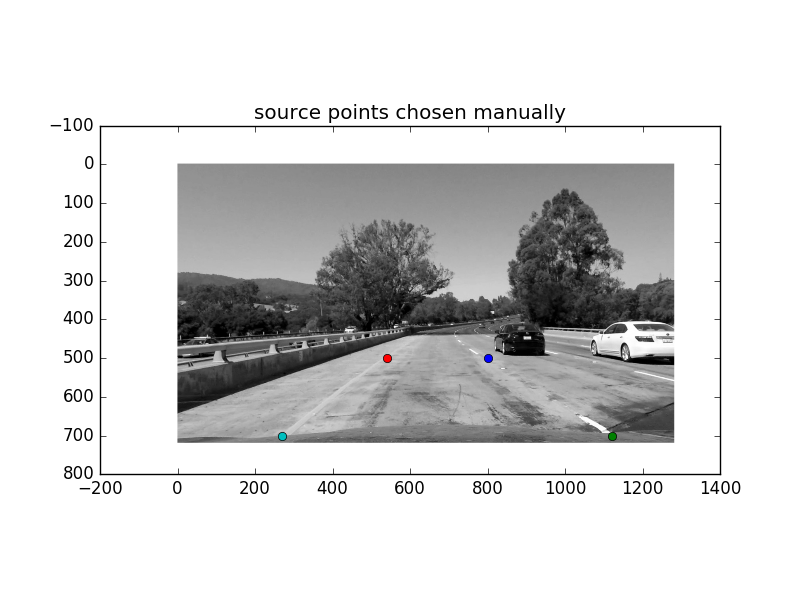
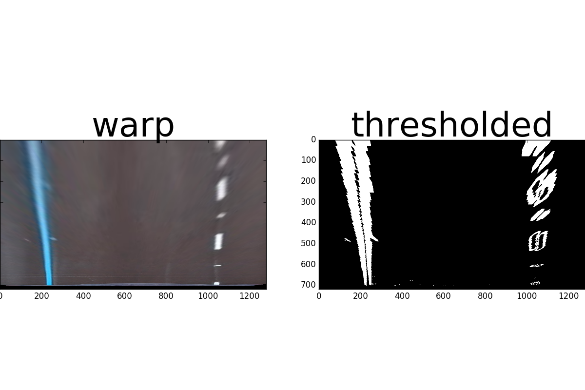
Then I chose four other points where I wanted to map my warped image to it. I applied cv2.getPerspectiveTransform to extract the transformation matrix M and unwrap transformation matrix Minv i.e. mapping from dst to src points. finally by using cv2.warpPerspective I warp the image. result of the warped imaged and corresponding binary image look like this:

4. Describe how (and identify where in your code) you identified lane-line pixels and fit their positions with a polynomial?

The code for below steps can be found in pipeline.py line 47 through 175.

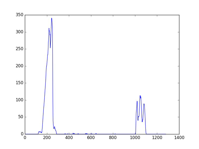
After lane lines are cleanly extracted, by scanning across x axis we can find peaks of accumulated pixels that helps us find lane lines. These peaks are a good identification of two lines, we can use it to place our starting point of our lines. histogram below visualise what I just explained:

For finding lines , It is a good idea to narrow down our searches vertical to the starting point images and focus on those area from bottom to top sliding like a window. I created 11 sliding windows with margin = 80 and minpx = 30 , to help set width with +/- margin and to recenter window if minimum pixel values not found in the window. Then on each iteration points are extracted for left and right line pixels While scanning from bottom to top bottom vertically and fit a second order polynomial curve for f(y) because lane lines in warped image are vertical. this process results like this:

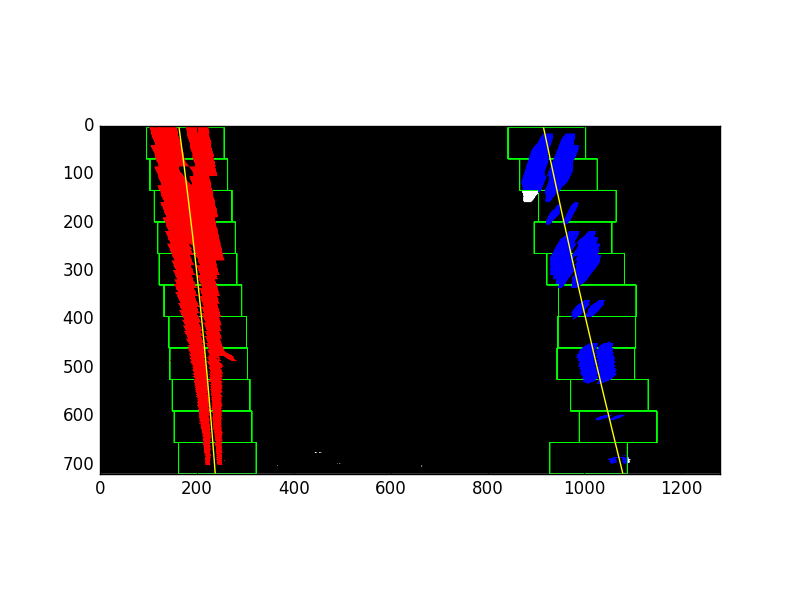
Above process is only triggered when detection the first frame of the video is occurred or when there are no line detected at all for either left or right side. After lines are detected Line class will track in memory coefficients for the last 15 frames and thereafter using numpy operations we average the best line of the last 15 iterations.

5. Describe how (and identify where in your code) you calculated the radius of curvature of the lane and the position of the vehicle with respect to centre.

I did this in lines 177 through 196 in my code in pipeline.py. For calculating radius of curvature having a second order polynomial I tried to fit a circle in y direction by calculation first and second derivative using curvature formula with respect to y direction, you may ask why y direction? well because we already know the lines are close to vertical in warped image and may have the same x value for more than one y value. I decided to chose maximum y value corresponding to bottom of image, this will help to measure curvature closest to the vehicle. This however gives pixel based values in pixel space. To make values make sense I needed to map pixel space values in pixel to real world space values preferably in meter unit. it is not a perfect accuracy however as It was not needed in this project ,I assumed conversion rate of 30 meters long and 3.7 meters wide.

6. Provide an example image of your result plotted back down onto the road such that the lane area is identified clearly.

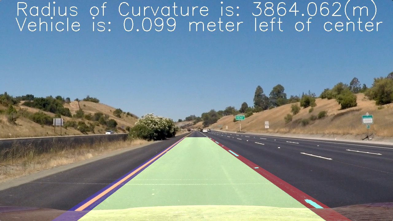
I implemented this step in lines 197 through 237 in my code in pipeline.py in lines . Here is an example of my result on a test image:

Pipeline (video)

1. Provide a link to your final video output. Your pipeline should perform reasonably well on the entire project video (wobbly lines are ok but no catastrophic failures that would cause the car to drive off the road!).

Here's a link to my video result

Discussion

1. Briefly discuss any problems / issues you faced in your implementation of this project. Where will your pipeline likely fail? What could you do to make it more robust?

Here I'll talk about the approach I took, what techniques I used, what worked and why, where the pipeline might fail and how I might improve it if I were going to pursue this project further.

Problems face and Recommandation for improvement

Right lane not found in the video: I had this issue while only using S channel, the top right points were not found when only thresholding only on S channel. I combined S channel with Sobel x operator and that solved the issue
Right Lane line in the beginning of the video is wobbly, thats because I slide the window on each frame. To solve this issue I recommend using a class that gets average of best line for 5 frames instead of each frame. Since lane lines in a video almost are the same per 5 to 10 frames.
If there is more time available to work on this project, you can also calculate an steering angel given the distance of vehicle to the lane line and radius of curvature.

Solved issues first iteration

Smoothing the line : over last 15 iteration and by getting average of the coefficients helps smoothen the line drawing on each frame
Faster and more robust search: Window search is only implemented once the frame is not detected at all, after that lanes will refer to their previous coordinates to place the starting line, this helped in robustness of the line
Calculating width of the lane in real space was statically that was set to 700 as width, now as suggested by a peer reviewer I replaced the width to dynamically be calculated from image shape and last determined coefficients, this helped in better drawing of the width in real world space.
Radius of curvature is checked and validated before drawing the line. Two lines are parallel if they have same slope, we check here if the ratio between radius of curvature of those two lines also making sense in terms of ratio. If the ratio of left/right line is smaller than 800 meter and the other left/right line is above 1000 (this gained empirically by debugging) we ditch the lines and use the last best fit.
Debugging video is added that is inspired by super handy suggestion by peer reviewer to debug outliers and observe behind the scenes
Line.py added to track all the lane lines and helped a lot to resolve smoothing and robustness issues.

Recommendation after first iteration

Combining the different threshold ratio of color, magnitude, direction, sober x and y and more other so that the shadows are completely removed and lines are finely detected. This is a very experimental step and by

solix/CarND-Advanced-Lane-Lines