The package FRK is now at v0.1.2 and available on CRAN! To install, please type
install.packages("FRK")To install the most recent (development) version, first please install INLA from http://www.r-inla.org/download, then please load devtools and type
install_github("andrewzm/FRK",dependencies=TRUE,build_vignettes=TRUE)A document containing a description, details on the underlying maths and computations, as well as several examples, is available as a vignette. To load this vignette please type
library(FRK)
vignette("FRK_intro")Package: FRK
Type: Package
Title: Fixed Rank Kriging
Version: 0.1.0
Date: 2016-04-19
Author: Andrew Zammit-Mangion
Maintainer: Andrew Zammit-Mangion andrewzm@gmail.com
Description: Fixed Rank Kriging is a tool for spatial/spatio-temporal modelling and prediction with large datasets. The approach, discussed in Cressie and Johannesson (2008), decomposes the field, and hence the covariance function, using a fixed set of n basis functions, where n is typically much smaller than the number of data points (or polygons) m. The method naturally allows for non-stationary, anisotropic covariance functions and the use of observations with varying support (with known error variance). The projected field is a key building block of the Spatial Random Effects (SRE) model, on which this package is based. The package FRK provides helper functions to model, fit, and predict using an SRE with relative ease. Reference: Cressie, N., & Johannesson, G. (2008). Fixed rank kriging for very large spatial data sets. Journal of the Royal Statistical Society: Series B, 70, 209-226.
License: GPL (>= 2)
library(sp)
library(ggplot2)
library(FRK)

## Setup
set.seed(1)                                               # Fix seed
zdf <- Z <- data.frame(x = runif(1000), y= runif(1000))   # Generate random locs
zdf$z <- Z$z <- sin(8*Z$x) + cos(8*Z$y) + 0.5*rnorm(100)  # Simulate data
coordinates(Z) = ~x+y                                     # Turn into sp object

## Run FRK
S <- FRK(f = z~1,                             # Formula to FRK
         list(Z),                             # All datasets are supplied in list
         n_EM = 10)                           # Max number of EM iterations
Pred <- SRE.predict(SRE_model = S)            # Prediction stage

xy <- data.frame(coordinates(Pred))           # Extract info from predictions
xy$mu <- Pred$mu
xy$se <- Pred$sd

## Plotting
ggplot(zdf) + geom_point(aes(x,y,colour=z)) +
             scale_colour_distiller(palette="Spectral") + theme_bw() + coord_fixed()
ggplot(xy) + geom_raster(aes(x,y,fill=mu)) +
             scale_fill_distiller(palette="Spectral") + theme_bw() + coord_fixed()
ggplot(xy) + geom_tile(aes(x,y,fill=se)) +
             geom_point(data=zdf,aes(x,y),pch=46) +
scale_fill_distiller(palette="Spectral") + theme_bw() + coord_fixed()//: # ( > ggsave(gdata,file="/Dropbox/Public/FRK/FRK_ex_data.png",width=7,height=5) > ggsave(gmu,file="/Dropbox/Public/FRK/FRK_ex_mu.png",width=7,height=5) > ggsave(gse,file="~/Dropbox/Public/FRK/FRK_ex_se.png",width=7,height=5) )
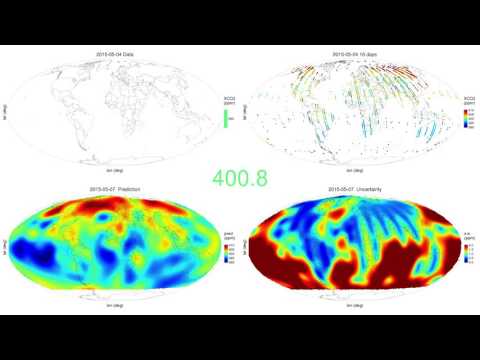
The package FRK is currently being used to generate spatio-temporal animations of fields observed by satellite data. Here we show a daily prediction of CO2 using data from the NASA OCO-2 between September 2014 and June 2016.


