A partial implementation of the CryoGrid permafrost model in Julia, with a focus on parameter estimation and uncertainty quantification.
Part of the broader research project: Quantifying and explaining uncertainty in permafrost modeling under a warming climate
Author: Brian Groenke (brian.groenke@awi.de)
- Fast and modular interface for defining multi-physics permafrost models including:
- Two-phase heat and water transport in porous media (i.e. soil and snow)
- Soil freeze-thaw dynamics from FreezeCurves.jl
- Surface energy balance
- Snow cover
- Salt diffusion
- Flexible interface for model parameter handling via ModelParameters.jl
- Support for automatic differentiation via ForwardDiff.jl
- Compatibility with ODE solvers OrdinaryDiffEq.jl as well as other SciML tools for analyzing dynamical systems
CryoGrid.jl can be installed via the Julia package manager:
add CryoGrid
or equivalently in code/REPL:
import Pkg
Pkg.add("CryoGrid")Here we define a multi-layer heat conduction model on the pre-defined soil profile for Samoylov Island.
Make sure that you have the Plots package installed in addition to CryoGrid in order to run this example code.
using CryoGrid
using Plots: plot

# load provided forcing data from Samoylov;
# The forcing file will be automatically downloaded to the input/ folder if not already present.
forcings = loadforcings(CryoGrid.Presets.Forcings.Samoylov_ERA_obs_fitted_1979_2014_spinup_extended_2044);
# get preset soil and initial temperature profile for Samoylov
soilprofile, tempprofile = CryoGrid.Presets.SamoylovDefault
initT = initializer(:T, tempprofile)
# choose grid with 5cm spacing
grid = CryoGrid.Presets.DefaultGrid_5cm
# build a default Tile with heat conduction on the given soil profile
tile = CryoGrid.Presets.SoilHeatTile(
    TemperatureBC(forcings.Tair),
    GeothermalHeatFlux(0.053u"W/m^2"),
    soilprofile,
    initT,
    grid=grid
)
# define time span (1 year)
tspan = (DateTime(2010,11,30),DateTime(2011,11,30))
u0, du0 = initialcondition!(tile, tspan)
# CryoGrid front-end for ODEProblem
prob = CryoGridProblem(tile, u0, tspan, savevars=(:T,))
# solve discretized system, saving every 3 hours
sol = @time solve(prob);
out = CryoGridOutput(sol)
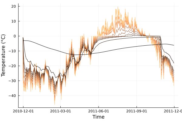
zs = [2,7,12,22,32,42,50,100,500]u"cm"
cg = Plots.cgrad(:copper,rev=true)
plot(out.T[Z(Near(zs))], color=cg[LinRange(0.0,1.0,length(zs))]', ylabel="Temperature", leg=false)The examples/ folder contains a number of other examples that should help users get started with the model.
In order to run these examples, it is recommended to clone the repository or add it as a development package via the package manager (i.e. dev CryoGrid instead of add CryoGrid). In the latter case, you can find the repository in $JULIA_HOME/.dev/CryoGrid.
Then cd into the CryoGrid repository and start julia with the examples folder set as the project environment; e.g. julia --project=examples or julia followed by activate examples in the package manager.
The package manager will install all additional dependencies needed for the examples (e.g. plotting and analysis packages). After this is finished, you should be able to run all of the examples without issue. If you encounter any errors while running the examples, please create an issue on GitHub so that we can fix it.
| CryoGrid Community (MATLAB) | CryoGrid3 (MATLAB) | CryoGridLite | CryoGrid.jl | |
|---|---|---|---|---|
| Heat conduction (enthalpy based) | ✅ | ❌ | ✅ | ✅ |
| Heat conduction (temperature based) | ❌ | ✅ | ❌ | ✅ |
| Soil freezing characteristics | ✅ | ✅ | ❌ | ✅ |
| Water balance, bucket advection | ✅ | ✅* | ❌ | ✅ |
| Water balance, Richard's equation | ✅ | ❌ | ❌ | ✅ |
| Snow, bulk (single-layer) | ❌ | ❌ | ❌ | ✅ |
| Snow, multi-layer, constant density | ✅ | ✅ | ✅ | 🚧 |
| Snow, multi-layer, w/ microphysics (CROCUS) | ✅ | ❌ | ❌ | ❌ |
| Surface energy balance, iterative | ✅ | ✅ | ❌ | ✅ |
| Surface energy balance, fully coupled | ❌ | ❌ | ❌ | ✅ |
| Evapotranspiration | ✅ | ✅ | ❌ | ✅ |
| Sublimation | ✅ | ✅ | ❌ | ❌ |
| Lake dynamics | ✅ | ❌ | ✅ | 🚧 |
| Salt diffusion | ✅ | ❌ | ❌ | ✅ |
| Lateral coupling, heat | ✅ | ✅ | ✅ | ❌ |
| Lateral coupling, water | ✅ | ✅ | ❌ | ❌ |
| Excess ice melt and subsidence | ✅ | ✅ | ❌ | ❌ |
| Excess ice aggradation | ✅ | ❌ | ❌ | ❌ |
| Vegetation dynamics | ✅ | ❌ | ❌ | ❌ |
| Overland flow | ✅ | ❌ | ❌ | ❌ |
| Surface infrastructure | ✅ | ❌ | ❌ | ❌ |
| Arbitrary time-varying boundary conditions | ❌ | ❌ | ❌ | ✅ |
| CryoGrid Community (MATLAB) | CryoGrid3 (MATLAB) | CryoGridLite | CryoGrid.jl | |
|---|---|---|---|---|
| Modular code structure | ✅ | ❌ | ❌ | ✅ |
| Ensemble simulations | ✅ | ❌ | ✅ | ✅ |
| Data assimilation and/or parameter estimation | ✅ | ❌ | ❌ | ✅ |
| Global sensitivity analysis | ❌ | ❌ | ❌ | ✅ |
| Higher-order numerical solvers | ❌ | ❌ | ❌ | ✅ |
| Automatic differentiation | ❌ | ❌ | ❌ | ✅ |
| Probabilistic programming and uncertainty quantification | ❌ | ❌ | ❌ | ✅ |
| ML emulator integration | ❌ | ❌ | ❌ | 🚧 |
| Automated testing framework | ❌ | ❌ | ❌ | ✅ |
| Non-proprietary runtime environment | ❌ | ❌ | ✅ | ✅ |

