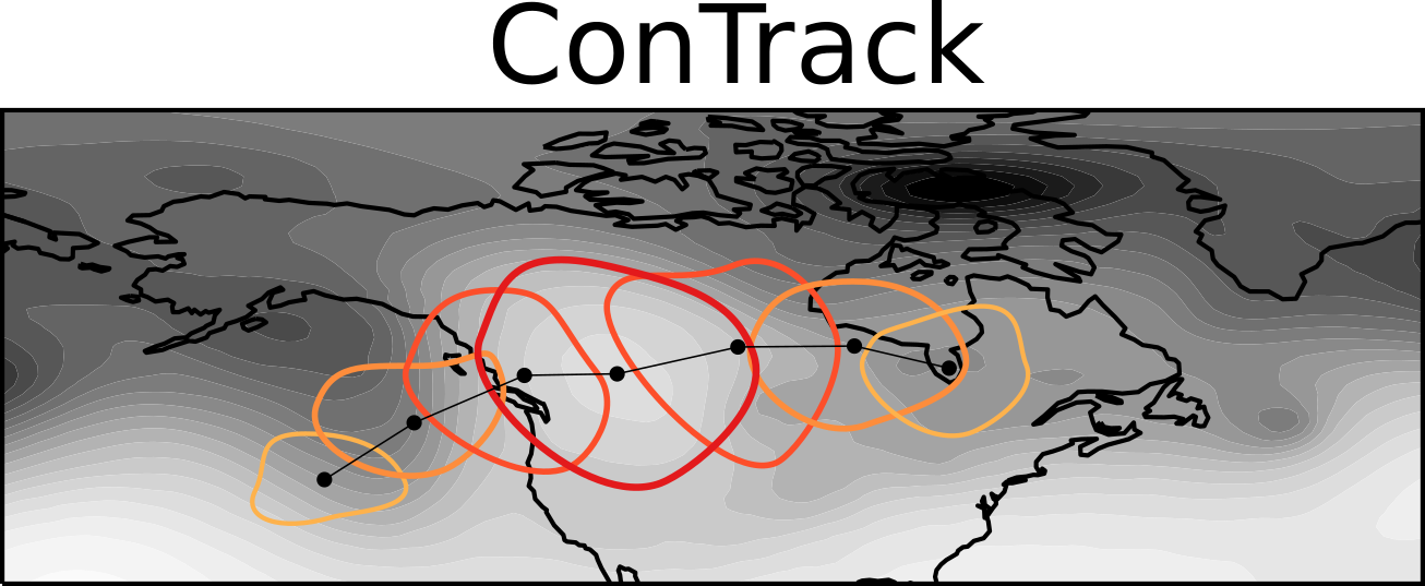
ConTrack is a Python package intended to simpify the process of automatically tracking and analyzing synoptic weather features (individual systems or long-term climatology) in weather and climate datasets. This feature-based tool is mostly used to track and characterize the life cycle of atmospheric blocking, but can also be used to identify other type of anomalous features, e.g., upper-level troughs and ridges (storm track). It is built on top of xarray and scipy.
ConTrack is based on the atmospheric blocking index by Schwierz et al. (2004) (written in Fortran) developed at the Institute for Atmospheric and Climate Science, ETH Zurich.
See also:
- Scherrer et al. (2005):
- Croci-Maspoli et al. (2007)
- Pfahl et al. (2015)
- Woollings et al. (2018)
- Steinfeld and Pfahl (2019)
- Steinfeld et al. (2020)
- and used in many more atmospheric blocking studies...
The ERA-Interim global blocking climatology based on upper-level potential vorticity used in Steinfeld and Pfahl (2019) is publicly available via an ETH Zurich-based web server [http://eraiclim.ethz.ch/ , see Sprenger et al. (2017)].
Ideally install it in a virtual environment (development version, master).
pip install git+https://github.com/steidani/ConTrack
Make sure you have the required dependencies (for details see docs/environment.yml):
- xarray
- scipy
- pandas
- numpy
- netCDF4
- (for plotting on geographical maps: matplotlib and cartopy)
- (for parallel computing: dask)
Copy/clone locally the latest version from ConTrack:
git clone git@github.com:steidani/ConTrack.git /path/to/local/contrack
cd path/to/local/contrack
Prepare the conda environment:
conda create -y -q -n contrack_dev python=3.8.5 pytest
conda env update -q -f docs/environment.yml -n contrack_dev
Install contrack in development mode in contrack_dev:
conda activate contrack_dev
pip install -e .
Run the tests:
python -m pytest
# import contrack module
from contrack import contrack

# initiate blocking instance
block = contrack()

# read ERA5 Z500 (geopotential at 500 hPa) daily global data from 19810101_00 to 20101231_00 with 1° spatial resolution)
# downloaded from https://cds.climate.copernicus.eu
block.read('data/era5_1981-2010_z_500.nc')
block
# Out[]:     Xarray dataset with 10957 time steps.
#            Available fields: z

# select only winter months January, February and December
block.ds = block.ds.sel(time=block.ds.time.dt.month.isin([1, 2, 12]))
# xarray.Dataset (and all its functions) can be accessed with block.ds

# calculate geopotential height
block.calculate_gph_from_gp(gp_name='z',
                            gp_unit='m**2 s**-2',
                            gph_name='z_height')

# Hint: Use block.set_up(...) to do consistency check and set (automatically or manually) names of dimension ('time', 'latitude', 'longitude')

# calculate Z500 anomaly (temporally smoothed with a 2 d running mean) with respect to the 31-day running mean (long-term: 30 years) climatology
block.calc_anom(variable='z_height',
                smooth=2,
                window=31,
                groupby='dayofyear')
# Hint: Use 'clim=...' to point towards an existing climatological mean (useful for weather forecasts)
# output: variable 'anom'.

# Finally, track blocking anticyclones (>=150gmp, 50% overlap twosided, 5 timesteps persistence (here 5 days))
block.run_contrack(variable='anom',
                   threshold=160,
                   gorl='>=',
                   overlap=0.5,
                   persistence=5,
                   twosided=True)
# output: variable 'flag'. 440 blocking systems tracked. Each blocking system is identified by a unique flag/ID.
block
# Out[]:     Xarray dataset with 2707 time steps.
#            Available fields: z, z_height, anom, flag

# Hint: In case you want to use a more objective threshold, e.g., the 90th percentile of the Z500 anomaly winter distribution over 50°-80°N, do:
# threshold = block['anom'].sel(latitude=slice(80, 50)).quantile([0.90], dim='time').mean() # 177gmp

# save to disk
block['flag'].to_netcdf('data/flag.nc')

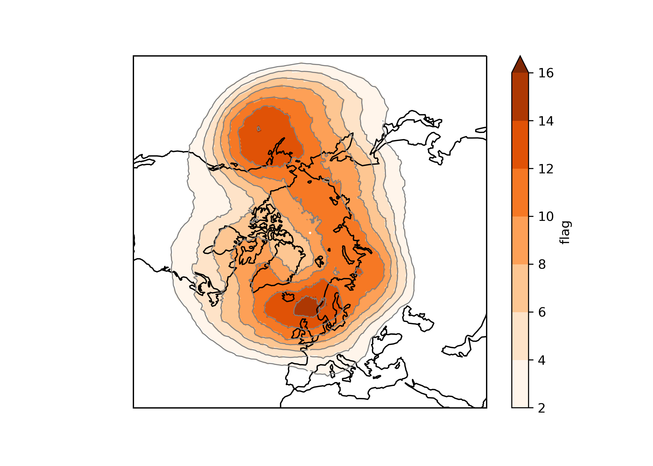
# plotting blocking frequency (in %) for winter over Northern Hemisphere
import matplotlib.pyplot as plt
import cartopy.crs as ccrs

fig, ax = plt.subplots(figsize=(7, 5), subplot_kw={'projection': ccrs.NorthPolarStereo()})
(xr.where(block['flag']>1,1,0).sum(dim='time')/block.ntime*100).plot(levels=np.arange(2,18,2), cmap='Oranges', extend = 'max', transform=ccrs.PlateCarree())
(xr.where(block['flag']>1,1,0).sum(dim='time')/block.ntime*100).plot.contour(colors='grey', linewidths=0.8, levels=np.arange(2,18,2), transform=ccrs.PlateCarree())
ax.set_extent([-180, 180, 30, 90], crs=ccrs.PlateCarree()); ax.coastlines();
plt.show()
Using the output 'flag' from block.run_contrack() to calculate blocking intensity, size, center of mass, age from genesis to lysis for each tracked feature.
# flag = output of block.run_contrack(), variable = input variable to calculate intensity and center of mass
block_df = block.run_lifecycle(flag='flag', variable='anom')

# output is a pandas.DataFrame
print(block_df)
           Flag         Date  Longitude  Latitude  Intensity        Size
     0        3  19810101_00        333        48     226.45  6490603.17
     1        3  19810102_00        335        47     210.77  6466790.05
     2        3  19810103_00        331        47     189.00  4169702.52
     3        3  19810104_00        331        49     190.78  3289504.87
     4        3  19810105_00        331        50     203.66  4231433.19
        ...          ...        ...       ...        ...         ...
     3832  6948  20101221_00        357       -53     206.02  5453454.76
     3833  6948  20101222_00          0       -56     208.80  5205585.69
     3834  6948  20101223_00          3       -56     190.23  6324017.70
     3835  6948  20101224_00          3       -57     214.02  5141693.22
     3836  6948  20101225_00          5       -55     211.33  7606108.76

# save result to disk
block_df.to_csv('data/block.csv', index=False)

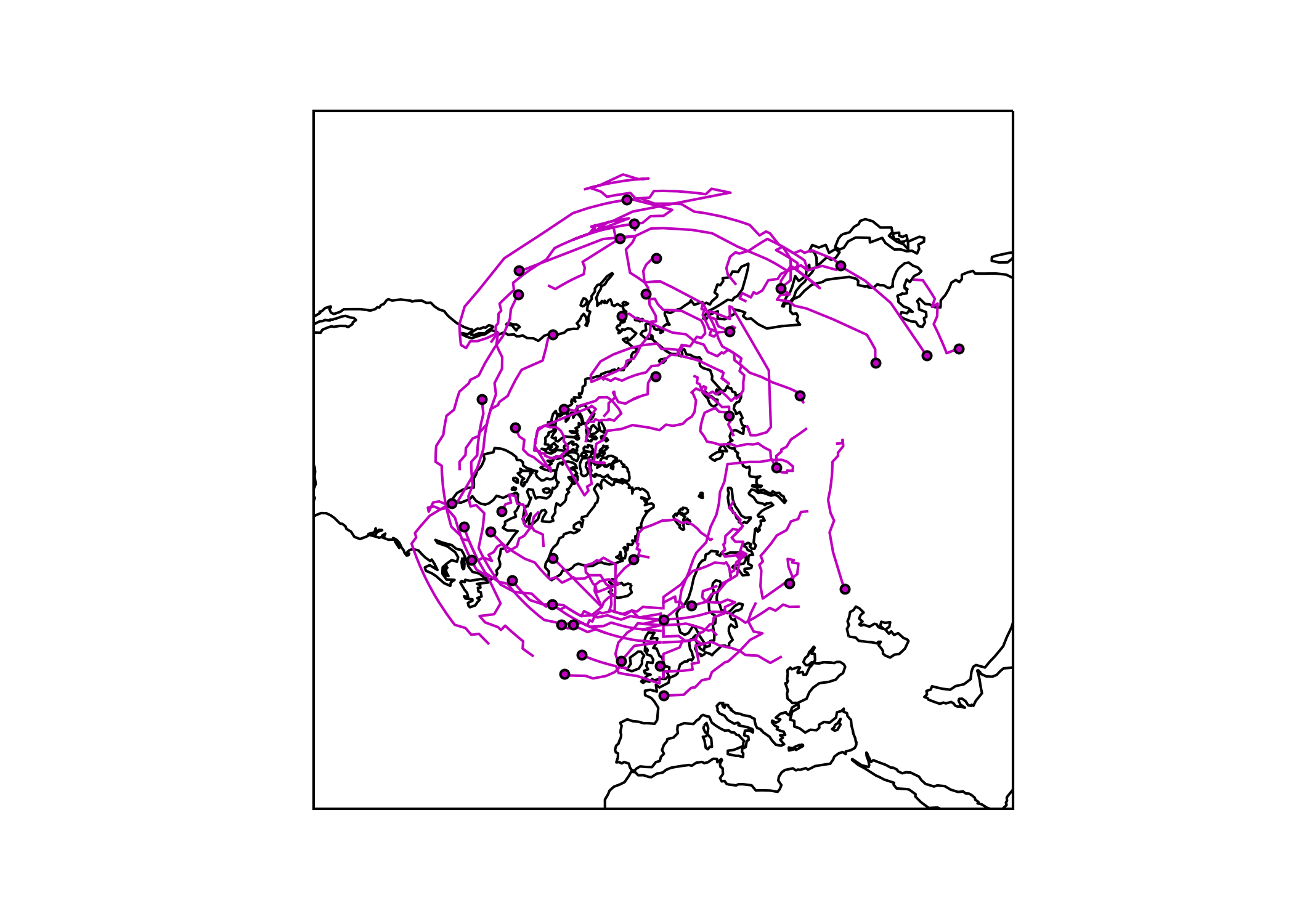
# plotting blocking track (center of mass) and genesis
f, ax = plt.subplots(1, 1, figsize=(7,5), subplot_kw=dict(projection=ccrs.NorthPolarStereo()))
ax.set_extent([-180, 180, 30, 90], crs=ccrs.PlateCarree()); ax.coastlines()
ax.coastlines() # add coastlines

#need to split each blocking track due to longitude wrapping (jumping at map edge)
for bid in np.unique(np.asarray(block_df['Flag'])): #select blocking id
    lons = np.asarray(block_df['Longitude'].iloc[np.where(block_df['Flag']==bid)])
    lats = np.asarray(block_df['Latitude'].iloc[np.where(block_df['Flag']==bid)])

    # cosmetic: sometimes there is a gap near map edge where track is split:
    lons[lons >= 355] = 359.9
    lons[lons <= 3] = 0.1
    segment = np.vstack((lons,lats))

    #move longitude into the map region and split if longitude jumps by more than "threshold"
    lon0 = 0 #center of map
    bleft = lon0-0.
    bright = lon0+360
    segment[0,segment[0]> bright] -= 360
    segment[0,segment[0]< bleft]  += 360
    threshold = 180  # CHANGE HERE
    isplit = np.nonzero(np.abs(np.diff(segment[0])) > threshold)[0]
    subsegs = np.split(segment,isplit+1,axis=+1)

    #plot the tracks
    for seg in subsegs:
        x,y = seg[0],seg[1]
        ax.plot(x ,y,c = 'm',linewidth=1, transform=ccrs.PlateCarree())
    #plot the starting points
    ax.scatter(lons[0],lats[0],s=11,c='m', zorder=10, edgecolor='black', transform=ccrs.PlateCarree())
- bugfix: how flag ID is tracked at periodic boundary.
- run_contrack(threshold): Threshold can now also be a xr.DataArray (1D) with time = 'dayofyear' to allow for variable threshold.
- bugfix: see Issue calc_clim error.
- first release on pypi
- calculate anomalies based on pre-defined climatology:
calc_anom(clim=...). - better handling of dimensions using
set_up()function. - twosided or forward overlap criterion:
run_contrack(twosided=True). run_lifecycle(): temporal evolution of intensity, spatial extent, center of mass and age from genesis to lysis for individual features.
- Extended functionality: Calculate anomalies from daily or monthly or seasonal... (long-term) climatology with moving average window:
calc_anom(groupby=..., window=...)


