This repo provides code for analyzing single-molecule spatial omics data and cell type location data using probabilistic indices. A simple use-case is shown below, more extensive documentation can be found in the vignette
The package can be installed from GitHub as follows:
library(devtools)
install_github("sthawinke/smoppix")
Once installed, you can load the package
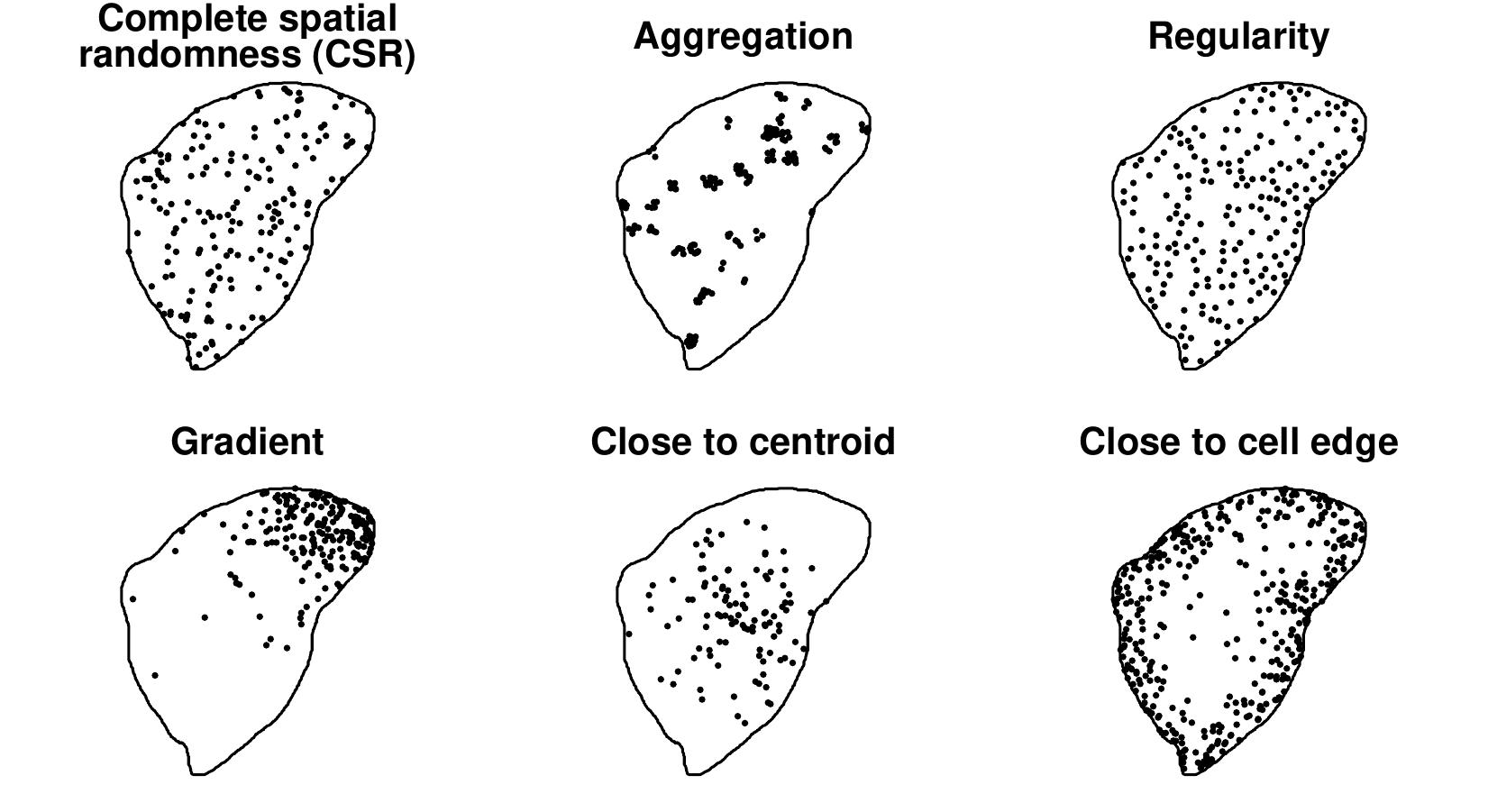
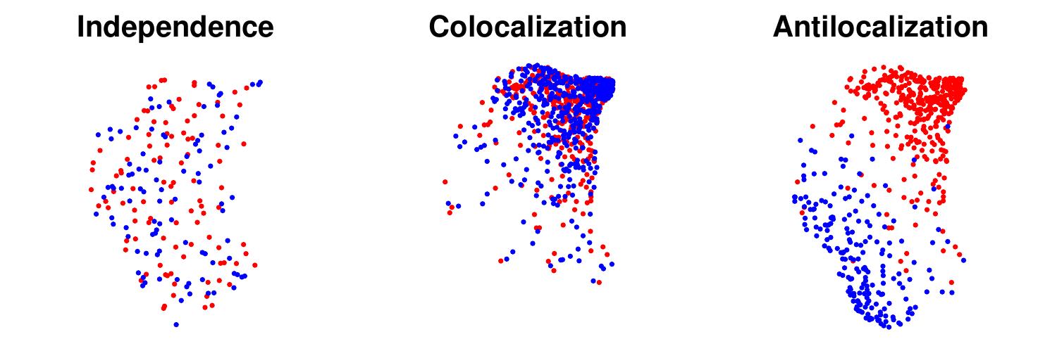
library(smoppix)Patterns that can be detected by smoppix:
For illustration, we now load an example dataset, contained in the package. It is in table format, so we first convert it to a spatstat hyperframe.
data(Yang)
hypYang <- buildHyperFrame(Yang,
    coordVars = c("x", "y"),
    imageVars = c("day", "root", "section")
)
## Found 29 unique images
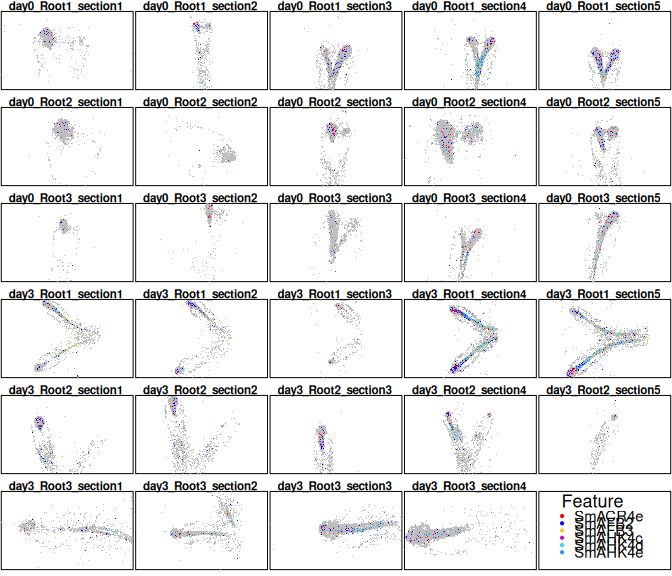
The number of unique images found is printed, make sure that this is what you expected. Now to make completely sure the software has understood us, we make an exploratory plot:
plotExplore(hypYang)As an example analysis, we estimate the univariate nearest neighbour probabilistic index as a measure of aggregation (clustering):
nnObj <- estPis(hypYang, pis = "nn", null = "background", verbose = FALSE)We add a variance weighting function to prepare for analysis and plot it:
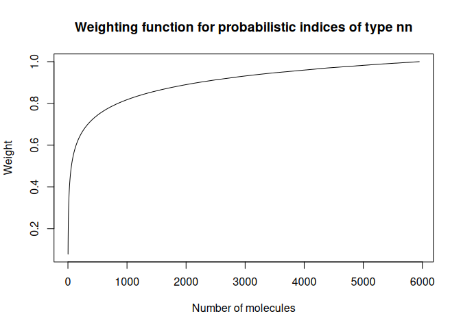
nnObj <- addWeightFunction(nnObj, designVars = c("day", "root"))
plotWf(nnObj, pi = "nn")
As expected, the weight allotted to the point pattern increases with the number of molecules in it: denser patterns provide more precise estimates of localization patterns.
Next is the inference step: we fit linear mixed models, and show the most significant results:
allModsNN <- fitLMMs(nnObj, fixedVars = "day", randomVars = "root")## Fitted formula for pi nn:
## pi - 0.5 ~ 1 + day + (1 | root)
head(getResults(allModsNN, "nn", "Intercept"))## Estimate SE pVal pAdj
## SmBIRDa 0.2631158 0.006767943 4.921471e-24 3.149742e-22
## SmAUX1a 0.3399689 0.005377353 3.527626e-22 1.128840e-20
## SmCYCA1;1a 0.3469608 0.006665333 2.995103e-19 6.389552e-18
## SmCYB2;4 0.3208844 0.008700097 4.881928e-18 7.811084e-17
## SmCYCD3;3a 0.3904109 0.005865331 5.676583e-17 7.266026e-16
## SmPFA2b 0.2250736 0.009834860 1.186476e-15 1.265574e-14
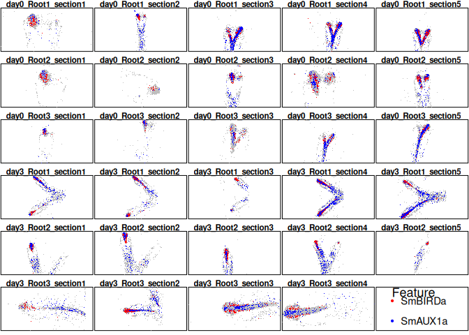
Let’s make it visual and plot the most significantly aggregated transcripts:
plotTopResults(hypYang, allModsNN, pi = "nn")Finally write the results to a spreadsheet:
writeToXlsx(allModsNN, file = "myfile.xlsx")
