High fidelity tomographic 3D printing

Files:

CAL_mp.py - python class for treating the 3D printing problem, starting from an STL file (CAL_mp uses multiprocessing unlike CAL.py)

*.ipynb - notebooks showing specific examples

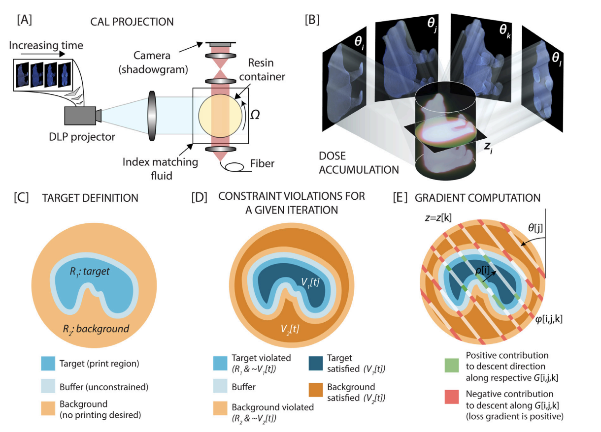
githubRepo_schematic.png - schematic showing the setup and conventions used to describe the problem

stlread_utils - folder containing STL file and temporary png slices

hollies_hand... - Folder containing output files for one particular geometry (note: the *.mat file containing projector inputs was deleted due to size)

tomoEnv.yml - environment file to run this project

Iterative projection calculation: forward model

This python implementation provides the optimization and projection generation framework used for volumetric additive manufacturing as described in the following publications:

[1] B. E. Kelly, I. Bhattacharya, H. Heidari, M. Shusteff, C. Spadaccini, H. K. Taylor, "Volumetric additive manufacturing via tomographic reconstruction", Science, 363 (6431), 1075-1079, 2019

[2] I. Bhattacharya, J. Toombs, H. K. Taylor, "High fidelity volumetric additive manufacturing", Additive Manufacturing, 47, 102299, 2021

[3] I. Bhattacharya, B. Kelly, M. Shusteff, C. Spadaccini, H. K. Taylor, "Computed axial lithography: volumetric 3D printing of arbitrary geometries", SPIE COSI, 2018

In computed axial lithography, a carefully calculated video is projected into a steadily rotating photocurable resin. The video is synchronized to the rotation of the resin so that specific images are projected at each rotated angle. This is modeled as an integral projection of the image through the resin container (in the low attenuation case). The accumulation of dose leads to a two step printing process. The first step, which consumes most of the dose, is an induction phase where oxygen free radicals are neutralized by polymer free radicals. The second step is gelation where the excess polymer free radicals cross-link and solidify into a desired geometry.

A detailed discussion and process model are provided in [1] and [2] above, but briefly, the forward model can be described as follows:

The 3D dose distribution within the photosensitive resin $f(\mathbf{r}, z)$ (Joules/cm3) arising from a set of projections $g(\rho, \theta, z)$ (Watt/cm2) can be expressed using the integral projection operation as:

$$ f(\mathbf{r}, z) = \frac{\alpha N_r}{\Omega} \int_{\theta = 0} ^{2\pi} g(\rho = \mathbf{r}.\hat{\theta}, \theta, z) e^{-\alpha \mathbf{r}. \hat{\theta}_\perp} d\theta $$

where $N_r$ denotes an integer number of rotations, $\alpha$ is the attenuation per unit length according to the Beer-Lambert law and $\Omega$ is the angular velocity of rotation of the resin container. Note that the expression excluding the pre-factor is the adjoint of the exponential radon tranform.

We are interested in achieving solidification in a region $R_1$ and no solidification in a subset of its compliment with respect to the region volume (which we denote as $R_2$). The dose requirement may be expressed in a simplified form as:

$$ R_1: f(\mathbf{r}, z) \ge d_h, R_2: f(\mathbf{r}, z) \le d_l $$

where $d_h > d_l$. Our goal is to calculate $g(\rho, \theta, z)$ that lead to $f(\mathbf{r}, z)$ that best satisfy the above conditions.

Optimization framework and software implementation

Figure: [A]: the hardware setup for 3D printing using a rotating resin container and projector, [B]: Schematic showing how different anges contribute to dose formation in 3D, [C]: the print target definition. Based on an input geometry, a target region, background and thin buffer region are created, [D]: Region definitions for computing the loss at any given iteration $t$, [E]: Gradient computation for the projector intensity values corresponding to a pixel $[i, j, k]$ in the projection space

Several possible mathematical optimization approaches could exist to encourage the print conditions as expressed in terms of $R_1$ and $R_2$ above. We focus on the penalty minimization (PM) approach as described in Ref. [2] above. The manuscript also explains how the PM approach is closely related to the iterative derivative-free optimization approach used in the first demonstration in Ref. [1]. In the PM approach, we seek to penalize any violations of the desired print target. Explicitly, regions where printing is desired but no printing occurs at optimization iteration $t$ are denoted as $\sim V_1[t]$. This is due to a lack of accumulated dose. Conversely, the region where printing is not desired but it occurs due to an excess of dose is denoted at $\sim V_2[t]$. An example of the region definitions for a particular z-slice are shown in the schematic D above.

We impose an L1 penalty on each of the types of violations and obtain the loss at iteration $t$ as follows:

$$ L_{PM}[t] = \int_{\sim V_2[t]} \left( \frac{N_r\alpha}{\Omega}(T^*_{-\alpha}[g](\mathbf{r})) - d_l \right) d\mathbf{r} $$

$$ - \int_{\sim V_1[t]} \left( \frac{N_r\alpha}{\Omega}(T^*_{-\alpha}[g](\mathbf{r})) - d_h \right) d\mathbf{r} $$

We would like to obtain $\hat{g}$ that minimizes this loss function. In order to implement a derivative based method to obtain the minimum, we calculate the gradient of this loss function with respect to a particular projector pixels intensity $G_{i,j,k}$:

$$ \frac{d L_{PM}[t]}{dG_{i,j,k}} = \int_{\sim V_2[t]} \frac{N_r \alpha}{\Omega}(T^{*}_{-\alpha}[\Gamma(i,j,k)](\mathbf{r})) d\mathbf{r} $$

$$ - \int_{\sim V_1[t]} \frac{N_r \alpha}{\Omega}(T^{*}_{-\alpha}[\Gamma(i,j,k)](\mathbf{r})) d\mathbf{r} $$

In the volume integrals above, the term corresponding to notation $\Gamma(i,j,k)$ indicates the volumetric exposure due to a single pixel indexed by $(i,j,k)$. For the purpose of this work, we model this using an integral projection (unfiltered inverse radon transform). The loss and gradient integrals are carried out using simple Riemann approximations with a particular grid size that can be selected.

The software implementation is through an optimization class CAL_mp. This uses multiprocessing for some of functions in order to speed up repetitive calculations that are applied over multiple z-slices. An example use case is provided in the notebook CAL_geometryIterations.ipynb. In order to initialize an optimization, we require the following inputs (in chronological order):

STL file of print target: placed user stlread_utils/STL_database
The order of the loss function (keep it 1 for L1 loss), parameters dl and dh for the optimization, size of angle discretization for the radon transform (361 here), lateral resolution of voxel grid to represent geometry (300 here)
Once the optimization object is initialized with these parameters using the CAL_mp class, we can set the parameters for the optimization. This uses the scipy.minimize class and related parameters (maxiter, ftol, disp, maxcor, maxls). The in-built LBFGS-B function is used to implement the optimization procedure.

The CAL_geometryIterations.ipynb notebook shows an example for optimizing the projections of a model of the COVID-19 virus. Once the optimization is complete, a graph of loss vs epochs and videos of various quantities of interest are created. The projections are saved as a matlab file ready for driving projector output.

The example below shows a set of outputs for the 3D printing of a prosthetic arm 'Hollie's hand'. This particular example is shown in the notebook CAL_example.ipynb for two sets of discretizations. Both of these led to perfect convergence (zero loss before iteration counts could be exhausted).

Please feel free to fork the repository and try it out with your own STL geometries.

Note: Perfect reconstruction in the imaging problem (even in the case of coarse angular sampling) has been studied, for example: E. Candes, J. Romberg, T. Tao, "Robust uncertainty principles: exact signal reconstruction from highly incomplete frequency information". The 3D printing problem is positivity constrained in the projection space, a significant difference and potential difficulty compared to the imaging problem. On an optimistic note, target geometries are often sparse and have highly sparse gradients (unlike the imaging problem) and the reconstruction problem is highly non-linear in dose. It would be interesting to study the parameter space of perfect reconstruction in the 3D printing problem.

finalProj.mp4

Acknowledgments

This work was carried out at the University of California Berkeley in the lab of Prof. Hayden Taylor. Please consider using this technology with intention towards socially beneficial and conscious projects. The examples used in this notebook: a prosthetic hand and a medical model, serve to illustrate some of the ways in which 3D printing can help our society. The models used here are under a creative commons license.

License

MIT Open Source License

Potential further steps

[1] Incorporate a more detailed forward model using Abbe imaging physics

[2] Discretization using the cylindrical symmetry of the problem or other non-uniform grids that could be beneficial

[3] Faster optimization methods or parallelization using a GPU