Python class for Multivariate Hawkes Processes

This repo provides a class MHP for doing basic experimentation with a Hawkes process. It works for both uni- and multivariate processes, and implements both synthetic sequence generation and parameter estimation of a known sequence. I use a MAP EM algorithm for parameter estimation that is described in this preprint and in a bit more detail in my masters thesis, both for the multivariate case. Please consider citing the preprint if you find the MAP EM approach helpful for your research, thank you!

There is a blog post here describing more details, such as theoretical preliminaries and some suggested usage and further reading.

The MHP.py file contains a single class, MHP. The core methods are:

generate_seq: generates synthetic sequences given parameter values specified in the constructor. Uses Ogata thinning with two speedups/modifications: it saves the rates at the moment of the last event, and it does the "attribution/rejection" test as a weighted random sample (using NumPy's random.sample) instead of, e.g., a for-loop.
EM: uses a Bayesian EM algorithm to learn parameters, given a sequence and estimates of alpha, mu, and omega. It treats omega as a hyperparameter and does not optimize over this parameter. For more details see the report, my thesis, or this blog post.

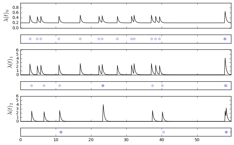
There are also two visualization methods, plot_events (which plots only the time series of events), and plot_rates (which plots the time series with the corresponding conditional intensities, currently only implemented for dim=3).

Usage

You can test basic functionality using default parameters as follows:

from MHP import MHP
P = MHP()
P.generate_seq(60)

which will initialize a univariate process with parameters mu=[0.1], alpha=[[0.5]], and omega=1.0. This sequence is stored as P.data, a numpy.ndarray with 2 columns: the first column with the timestamps, the second with the stream assignment (in this case there is only one stream).

You can then plot the events with

P.plot_events()

For a more interesting test, try engineering your own parameters. Here is an example with dim=3:

m = np.array([0.2, 0.0, 0.0])
a = np.array([[0.1, 0.0, 0.0], 
              [0.9, 0.0, 0.0],
              [0.0, 0.9, 0.0]])
w = 3.1

P = MHP(mu=m, alpha=a, omega=w)
P.generate_seq(60)
P.plot_events()

We can also look at the conditional intensities along with the time series of events:

We can learn the parameters of an already generated sequence by simply calling EM with some guesses at alpha and mu (and a hyperparameter omega),

mhat = np.random.uniform(0,1, size=3)
ahat = np.random.uniform(0,1, size=(3,3))
w = 3.

P.EM(ahat, mhat, w)

which will give output something like:

After ITER 0 (old: -10000.000 new: -0.129)
 terms 5.1766, 17.4638, 8.5362
After ITER 10 (old: -0.129 new: -1.349)
 terms -20.8908, 11.8172, 14.1828
Reached stopping criterion. (Old: -1.349 New: -1.350)

(array([[ 0.0223,  0.1475,  0.    ],
        [ 0.5954,  0.    ,  0.    ],
        [ 0.    ,  0.625 ,  0.    ]]), 
 array([ 0.2038,  0.0046,  0.    ]))

This is already a reasonable approximation to the actual ground truth values from above, without including regularization, cross-validation, a larger sample, etc.

Summary

This is a bare bones collection of code that is hopefully helpful to someone dipping his/her toes in the waters of multivariate point processes. For more robust packages, or a more indepth look at behind-the-scenes, check out this blog post which covers some basic theoretical concepts and also links to some other more expansive code repos out there.

stmorse/hawkes

Python class for Multivariate Hawkes Processes

Contents

Usage

Summary