Foundry is a package for forging interpretable predictive modeling pipelines with a sklearn style-API. It includes:
- A
Glmclass with a Pytorch backend. This class is highly extensible, supporting (almost) any distribution in pytorch's distributions module. - A
preprocessingmodule that includes helpful classes likeDataFrameTransformerandInteractionFeatures. - An
evaluationmodule with tools for interpreting any sklearn-API model viaMarginalEffects.
You should use Foundry to augment your workflows if any of the following are true:
- You are attempting to model a target that is 'weird': for example, highly skewed data, binomial count-data, censored or truncated data, etc.
- You need some help battling some annoying aspects of feature-engineering: for example, you want an expressive way of specifying interaction-terms in your model; or perhaps you just want consistent support for getting feature-names despite being stuck on python 3.7.
- You want to interpret your model: for example, perform statistical inference on its parameters, or understand the direction and functional-form of its predictors.
foundry can be installed with pip:
pip install git+https://github.com/strongio/foundry.git#egg=foundryLet's walk through a quick example:
# data:
from foundry.data import get_click_data
# preprocessing:
from foundry.preprocessing import DataFrameTransformer, SimpleImputer
from sklearn.preprocessing import OneHotEncoder, StandardScaler, PowerTransformer
from sklearn.pipeline import make_pipeline
# glm:
from foundry.glm import Glm
# evaluation:
from foundry.evaluation import MarginalEffects
Here's a dataset of click user pageviews and clicks for domain with lots of pages:
df_train, df_val = get_click_data()
df_train| attributed_source | user_agent_platform | page_id | page_market | page_feat1 | page_feat2 | page_feat3 | num_clicks | num_views | |
|---|---|---|---|---|---|---|---|---|---|
| 0 | 8 | Windows | 7 | b | 0.0 | 0.0 | 35.0 | 0.0 | 32.0 |
| 1 | 8 | Windows | 7 | b | 0.0 | 1.0 | 0.0 | 0.0 | 14.0 |
| 2 | 8 | Windows | 7 | a | 0.0 | 0.0 | 5.0 | 0.0 | 8.0 |
| 3 | 8 | Windows | 7 | a | 0.0 | 0.0 | 9.0 | 0.0 | 7.0 |
| 4 | 8 | Windows | 7 | a | 0.0 | 0.0 | 20.0 | 0.0 | 40.0 |
| ... | ... | ... | ... | ... | ... | ... | ... | ... | ... |
| 423188 | 1 | Android | 95 | f | 0.0 | 0.0 | 25.0 | 0.0 | 1.0 |
| 423189 | 10 | Android | 26 | a | 0.0 | 2.0 | 7.0 | 15.0 | 860.0 |
| 423190 | 10 | Android | 32 | a | 0.0 | 0.0 | 36.0 | 37.0 | 651.0 |
| 423191 | 0 | Other | 10 | b | 0.0 | 0.0 | 26.0 | 0.0 | 1.0 |
| 423192 | 0 | Other | 31 | a | 0.0 | 1.0 | 34.0 | 0.0 | 1.0 |
423193 rows × 9 columns
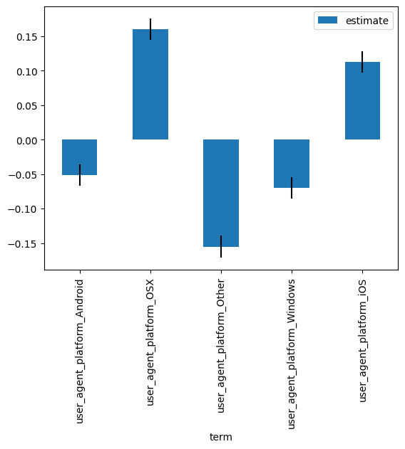
We'd like to build a model that let's us predict future click-rates for different pages (page_id), page-attributes (e.g. market), and user-attributes (e.g. platform), and also learn about each of these features -- e.g. perform statistical inference on model-coefficients ("are users with missing user-agent data significantly worse than average?")
Unfortunately, these data don't fit nicely into the typical regression/classification divide: each observations captures counts of clicks and counts of pageviews. Our target is the click-rate (clicks/views) and our sample-weight is the pageviews.
One workaround would be to expand our dataset so that each row indicates is_click (True/False) -- then we could use a standard classification algorithm:
df_train_expanded, df_val_expanded = get_click_data(expanded=True)
df_train_expanded| attributed_source | user_agent_platform | page_id | page_market | page_feat1 | page_feat2 | page_feat3 | is_click | |
|---|---|---|---|---|---|---|---|---|
| 0 | 8 | Windows | 67 | b | 0.0 | 1.0 | 0.0 | False |
| 1 | 8 | Windows | 67 | b | 0.0 | 1.0 | 0.0 | False |
| 2 | 8 | Windows | 67 | b | 0.0 | 1.0 | 0.0 | False |
| 3 | 8 | Windows | 67 | b | 0.0 | 1.0 | 0.0 | False |
| 4 | 8 | Windows | 67 | b | 0.0 | 1.0 | 0.0 | False |
| ... | ... | ... | ... | ... | ... | ... | ... | ... |
| 7760666 | 7 | OSX | 61 | c | 3.0 | 1.0 | 12.0 | False |
| 7760667 | 7 | OSX | 61 | c | 3.0 | 1.0 | 12.0 | False |
| 7760668 | 7 | OSX | 61 | c | 3.0 | 1.0 | 12.0 | False |
| 7760669 | 7 | OSX | 61 | c | 3.0 | 1.0 | 12.0 | False |
| 7760670 | 7 | OSX | 61 | c | 3.0 | 1.0 | 12.0 | False |
7760671 rows × 8 columns
But this is hugely inefficient: our dataset of ~400K explodes to almost 8MM.
Within foundry, we have the Glm, which supports binomial data directly:
Glm('binomial', penalty=10_000)Glm(family='binomial', penalty=10000)
Let's set up a sklearn model pipeline using this Glm. We'll use foundry's DataFrameTransformer to support passing feature-names to the Glm (newer versions of sklearn support this via the set_output() API).
preproc = DataFrameTransformer([
    (
        'one_hot',
        make_pipeline(SimpleImputer(strategy='most_frequent'), OneHotEncoder()),
        ['attributed_source', 'user_agent_platform', 'page_id', 'page_market']
    )
    ,
    (
        'power',
        PowerTransformer(),
        ['page_feat1', 'page_feat2', 'page_feat3']
    )
])
glm = make_pipeline(
preproc,
Glm('binomial', penalty=1_000)
).fit(
X=df_train,
y={
'value' : df_train['num_clicks'],
'total_count' : df_train['num_views']
},
)Epoch 8; Loss 0.3183; Convergence 0.0003131/0.001: 42%|█████▊ | 5/12 [00:00<00:00, 10.99it/s]
Estimating laplace coefs... (you can safely keyboard-interrupt to cancel)
Epoch 8; Loss 0.3183; Convergence 0.0003131/0.001: 42%|█████▊ | 5/12 [00:07<00:10, 1.55s/it]
By default, the Glm will estimate not just the parameters of our model, but also the uncertainty associated with them. We can access a dataframe of these with the coef_dataframe_ attribute:
df_coefs = glm[-1].coef_dataframe_
df_coefs| name | estimate | se | |
|---|---|---|---|
| 0 | probs__one_hot__attributed_source_0 | 0.000042 | 0.031622 |
| 1 | probs__one_hot__attributed_source_1 | -0.003277 | 0.031578 |
| 2 | probs__one_hot__attributed_source_2 | -0.058870 | 0.030623 |
| 3 | probs__one_hot__attributed_source_3 | -0.485669 | 0.024011 |
| 4 | probs__one_hot__attributed_source_4 | -0.663989 | 0.016975 |
| ... | ... | ... | ... |
| 141 | probs__one_hot__page_market_z | 0.353556 | 0.025317 |
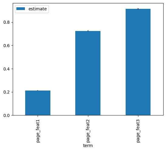
| 142 | probs__power__page_feat1 | 0.213486 | 0.002241 |
| 143 | probs__power__page_feat2 | 0.724601 | 0.004021 |
| 144 | probs__power__page_feat3 | 0.913425 | 0.004974 |
| 145 | probs__bias | -5.166077 | 0.022824 |
146 rows × 3 columns
Using this, it's easy to plot our model-coefficients:
df_coefs[['param', 'trans', 'term']] = df_coefs['name'].str.split('__', n=3, expand=True)

df_coefs[df_coefs['name'].str.contains('page_feat')].plot('term', 'estimate', kind='bar', yerr='se')
df_coefs[df_coefs['name'].str.contains('user_agent_platform')].plot('term', 'estimate', kind='bar', yerr='se')
<AxesSubplot:xlabel='term'>
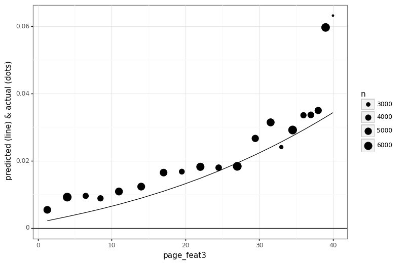
Model-coefficients are limited because they only give us a single number, and for non-linear models (like our binomial GLM) this doesn't tell the whole story. For example, how could we translate the importance of page_feat3 into understanable terms? This only gets more difficult if our model includes interaction-terms.
To aid in this, there is MarginalEffects, a tool for plotting our model-predictions as a function of each predictor:
glm_me = MarginalEffects(glm)
glm_me.fit(
    X=df_val_expanded,
    y=df_val_expanded['is_click'],
    vary_features=['page_feat3']
).plot()
<ggplot: (8777751556441)>
Here we see that how this predictor's impact on click-rates varies due to floor effects.
As a bonus, we plotted the actual values alongside the predictions, and we can see potential room for improvement in our model: it looks like very high values of this predictor have especially high click-rates, so an extra step in feature-engineering that captures this discontinuity may be warranted.


