Frequently in data science, we have a relationship between X and y where (probabilistically) y increases as X does.
There is a classical algorithm for solving this problem nonparametrically, specifically Isotonic regression. This simple algorithm is also implemented in sklearn.isotonic. The classic algorithm is based on a piecewise constant approximation - with nodes at every data point - as well as minimizing (possibly weighted) l^2 error.
I'm a heavy user of isotonic regression, but unfortunately the version in sklearn does not meet my needs. Specific failings:
- My data is frequently binary. This means that each
y[i]is either 0 or 1, but the probability thaty[i]==1increasers asx[i]increases. - My data is often noisy with fatter than normal tails, which means that minimizing
l^2error overweights outliers. - The size of the isotonic model is large -
O(N), in fact (withNthe size of the training data). - The curves output by sklearn's isotonic model are piecewise constant with a large number of discontinuities (
O(N)of them).
This library is an attempt to solve these problems once and for all.
More info on details and motivation is described in a companion blog post.
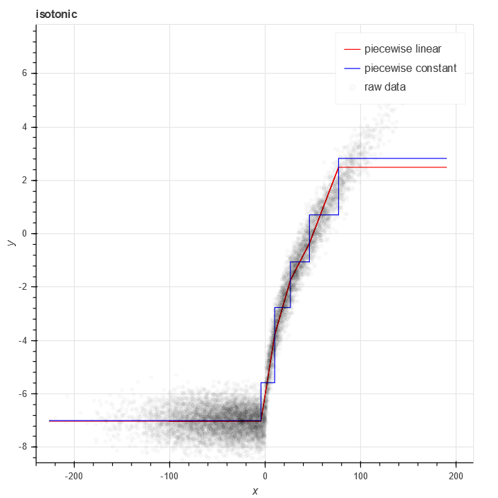
To fit a curve to real valued data using mean squared error, it's it's pretty straightforward:
from scipy.stats import norm, bernoulli
import numpy as np

N = 10000
x = norm(0,50).rvs(N) - bernoulli(0.25).rvs(N)*50
y = -7+np.sqrt(np.maximum(x, 0)) + norm(0,0.5).rvs(N)

from isotonic import LpIsotonicRegression
from isotonic.curves import PiecewiseLinearIsotonicCurve, PiecewiseConstantIsotonicCurve

import pandas as pd
from bokeh.plotting import figure, output_notebook, show
from bokeh.models import Span, LinearAxis, Range1d, ColumnDataSource
output_notebook()

plot = figure(
    tools="pan,box_zoom,reset,save,",
    y_axis_label="y", title="isotonic",
    x_axis_label='x'
)

curve = LpIsotonicRegression(10, increasing=True, curve_algo=PiecewiseLinearIsotonicCurve).fit(x, y)
curve2 = LpIsotonicRegression(10, increasing=True, curve_algo=PiecewiseConstantIsotonicCurve).fit(x, y)
#curve = PiecewiseIsotonicCurve(x_cuts, gamma_of_alpha(result.x))
xx = np.arange(x.min(), x.max(), 0.01)
plot.line(xx, curve.predict_proba(xx), color='red', legend_label='piecewise linear')
plot.line(xx, curve2.predict_proba(xx), color='blue', legend_label='piecewise constant')

plot.circle(x, y, color='black', alpha=0.02, legend_label='raw data')

show(plot)
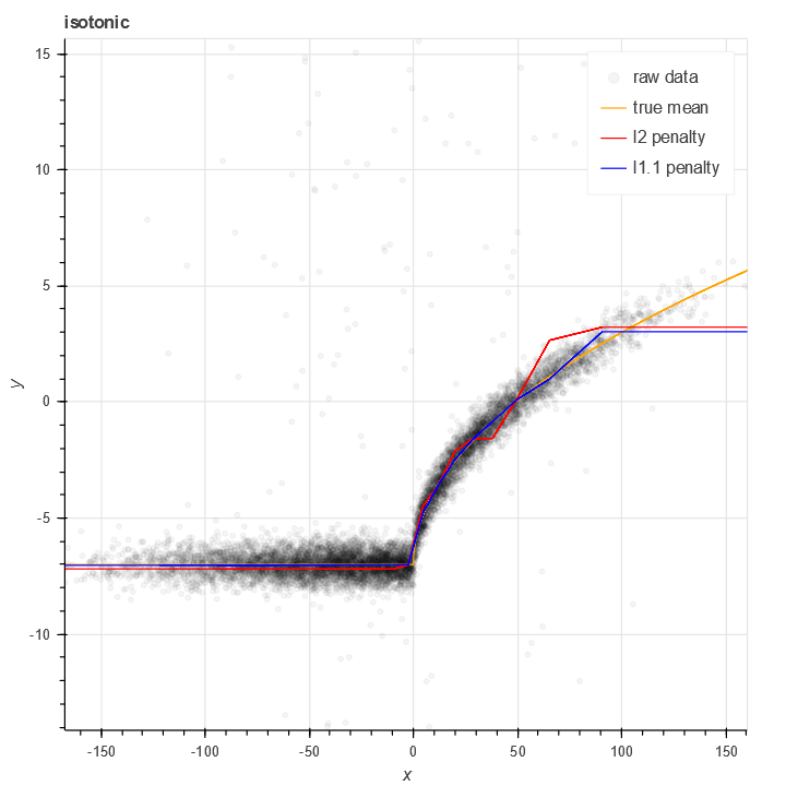
Like most regression methods based on l^2 loss, isotonic regression is sensitive to noise. As the name LpIsotonicRegression suggests, one can use alternate powers to accomodate greater degrees of noise. Consider the same example as above, but 5% of the samples are corrupted by high intensity Laplacian noise:
y = -7+np.sqrt(np.maximum(x, 0)) + norm(0,0.5).rvs(N) + bernoulli(0.05).rvs(N) * laplace(scale=50).rvs(N)
We can compare the result of LpIsotonicRegression with different powers. Choosing an norm l^p for p nearly 1 yields a fit significantly less sensitive:
curve = LpIsotonicRegression(20, power=2, increasing=True, curve_algo=PiecewiseLinearIsotonicCurve).fit(x, y)
curve2 = LpIsotonicRegression(20, power=1.1, increasing=True, curve_algo=PiecewiseLinearIsotonicCurve).fit(x, y)
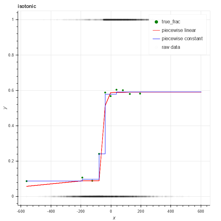
In many cases the data I wish to handle is binary, not real valued. That is, every y[i] is either 0 or 1. The value I wish to estimate is the probability that y == 1, given a value of x.
In isotonic, this is handled with the BinomialIsotonicRegression class. This fits a curve to binary data based on a binomial loss function.
from isotonic import BinomialIsotonicRegression
from isotonic.curves import PiecewiseLinearIsotonicCurve, PiecewiseConstantIsotonicCurve

import pandas as pd
from bokeh.plotting import figure, output_notebook, show
from bokeh.models import Span, LinearAxis, Range1d, ColumnDataSource
output_notebook()

plot = figure(
    tools="pan,box_zoom,reset,save,",
    y_axis_label="y", title="isotonic",
    x_axis_label='x'
)

M = 10
x_cuts = np.quantile(x, np.arange(0,1,1/M))
df = pd.DataFrame({'x': x, 'y': y, 'x_c': x_cuts[np.digitize(x, x_cuts)-1]})
grouped = df.groupby('x_c')['y'].mean().reset_index()

plot.circle(grouped['x_c'], grouped['y'], color='green', legend_label='true_frac')

curve = BinomialIsotonicRegression(10, increasing=True, curve_algo=PiecewiseLinearIsotonicCurve).fit(x, y)
curve2 = BinomialIsotonicRegression(10, increasing=True, curve_algo=PiecewiseConstantIsotonicCurve).fit(x, y)

xx = np.arange(x.min(), x.max(), 0.01)
plot.line(xx, curve.predict_proba(xx), color='red', legend_label='piecewise linear')
plot.line(xx, curve2.predict_proba(xx), color='blue', legend_label='piecewise constant')

plot.circle(x, y, color='black', alpha=0.01, legend_label='raw data')
show(plot)


