PyTorch implementation of the InfoNCE loss from "Representation Learning with Contrastive Predictive Coding". In contrastive learning, we want to learn how to map high dimensional data to a lower dimensional embedding space. This mapping should place semantically similar samples close together in the embedding space, whilst placing semantically distinct samples further apart. The InfoNCE loss function can be used for the purpose of contrastive learning.
This package is available on PyPI and can be installed via:
pip install info-nce-pytorch
Can be used without explicit negative keys, whereby each sample is compared with the other samples in the batch.
loss = InfoNCE()
batch_size, embedding_size = 32, 128
query = torch.randn(batch_size, embedding_size)
positive_key = torch.randn(batch_size, embedding_size)
output = loss(query, positive_key)
Can be used with negative keys, whereby every combination between query and negative key is compared.
loss = InfoNCE(negative_mode='unpaired') # negative_mode='unpaired' is the default value
batch_size, num_negative, embedding_size = 32, 48, 128
query = torch.randn(batch_size, embedding_size)
positive_key = torch.randn(batch_size, embedding_size)
negative_keys = torch.randn(num_negative, embedding_size)
output = loss(query, positive_key, negative_keys)
Can be used with negative keys, whereby each query sample is compared with only the negative keys it is paired with.
loss = InfoNCE(negative_mode='paired')
batch_size, num_negative, embedding_size = 32, 6, 128
query = torch.randn(batch_size, embedding_size)
positive_key = torch.randn(batch_size, embedding_size)
negative_keys = torch.randn(batch_size, num_negative, embedding_size)
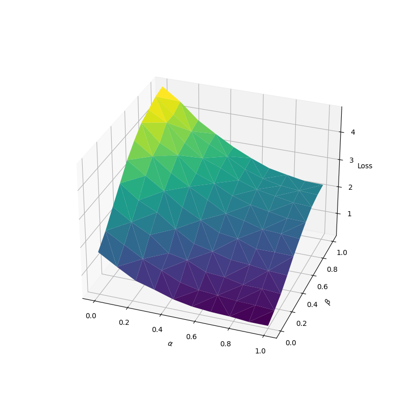
output = loss(query, positive_key, negative_keys)Suppose we have some initial mean vectors µ_q, µ_p, µ_n and a covariance matrix Σ = I/10, then we can plot the value of the InfoNCE loss by sampling from distributions with interpolated mean vectors.
Given interpolation weights α and β, we define the distribution Q ~ N(µ_q, Σ) for the query samples, the distribution P_α ~ N(αµ_q + (1-α)µ_p, Σ) for the positive samples
and the distribution N_β ~ N(βµ_q + (1-β)µ_n, Σ) for the negative samples.
Shown below is the value of the loss with inputs sampled from the distributions defined above for different values of α and β.
