d3-hierarchy

Many datasets are intrinsically hierarchical. Consider geographic entities, such as census blocks, census tracts, counties and states; the command structure of businesses and governments; file systems and software packages. And even non-hierarchical data may be arranged empirically into a hierarchy, as with k-means clustering or phylogenetic trees.

This module implements several popular techniques for visualizing hierarchical data:

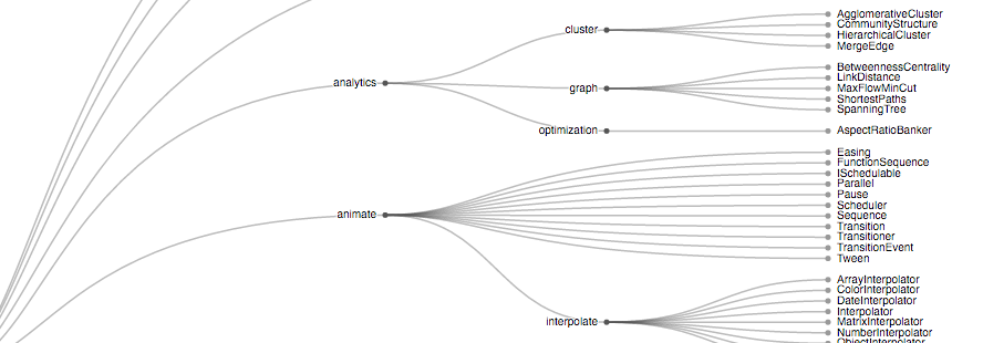
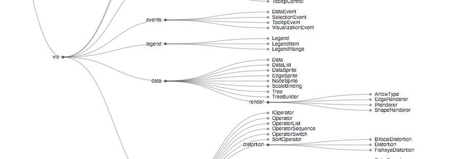
Node-link diagrams show topology using discrete marks for nodes and links, such as a circle for each node and a line connecting each parent and child. The “tidy” tree is delightfully compact, while the dendrogram places leaves at the same level. (These have both polar and Cartesian forms.) Indented trees are useful for interactive browsing.

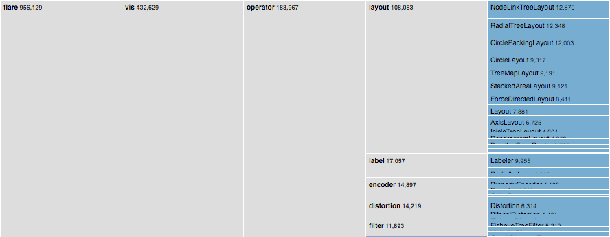
Adjacency diagrams show topology through the relative placement of nodes. They may also encode a quantitative dimension in the area of each node, for example to show revenue or file size. The “icicle” diagram uses rectangles, while the “sunburst” uses annular segments.

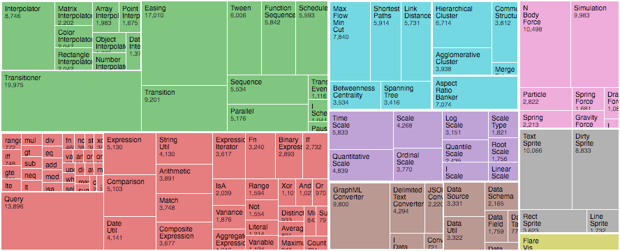
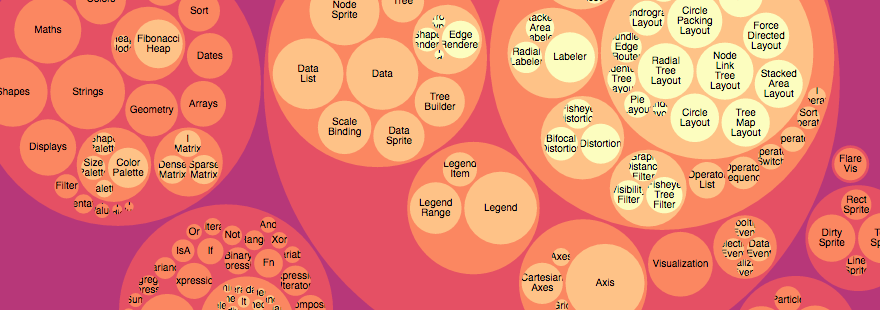
Enclosure diagrams also use an area encoding, but show topology through containment. A treemap recursively subdivides area into rectangles. Circle-packing tightly nests circles; this is not as space-efficient as a treemap, but perhaps more readily shows topology.

A good hierarchical visualization facilitates rapid multiscale inference: micro-observations of individual elements and macro-observations of large groups.

Installing

If you use NPM, npm install d3-hierarchy. Otherwise, download the latest release. You can also load directly from d3js.org, either as a standalone library or as part of D3 4.0. AMD, CommonJS, and vanilla environments are supported. In vanilla, a d3 global is exported:

<script src="https://d3js.org/d3-hierarchy.v1.min.js"></script>
<script>

var treemap = d3.treemap();

</script>

Try d3-hierarchy in your browser.

Hierarchy

Before you can compute a hierarchical layout, you need a root node. If your data is already in a hierarchical format, such as JSON, you can pass it directly to d3.hierarchy; otherwise, you can rearrange tabular data, such as comma-separated values (CSV), into a hierarchy using d3.stratify.

# d3.hierarchy(data[, children]) <>

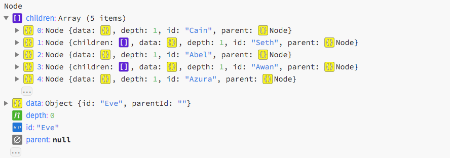
Constructs a root node from the specified hierarchical data. The specified data must be an object representing the root node. For example:

{
  "name": "Eve",
  "children": [
    {
      "name": "Cain"
    },
    {
      "name": "Seth",
      "children": [
        {
          "name": "Enos"
        },
        {
          "name": "Noam"
        }
      ]
    },
    {
      "name": "Abel"
    },
    {
      "name": "Awan",
      "children": [
        {
          "name": "Enoch"
        }
      ]
    },
    {
      "name": "Azura"
    }
  ]
}

The specified children accessor function is invoked for each datum, starting with the root data, and must return an array of data representing the children, or null if the current datum has no children. If children is not specified, it defaults to:

function children(d) {
  return d.children;
}

The returned node and each descendant has the following properties:

node.data - the associated data, as specified to the constructor.
node.depth - zero for the root node, and increasing by one for each descendant generation.
node.height - zero for leaf nodes, and the greatest distance from any descendant leaf for internal nodes.
node.parent - the parent node, or null for the root node.
node.children - an array of child nodes, if any; undefined for leaf nodes.
node.value - the summed value of the node and its descendants; optional, see node.sum and node.count.

This method can also be used to test if a node is an instanceof d3.hierarchy and to extend the node prototype.

# node.ancestors() <>

Returns the array of ancestors nodes, starting with this node, then followed by each parent up to the root.

# node.descendants() <>

Returns the array of descendant nodes, starting with this node, then followed by each child in topological order.

# node.leaves() <>

Returns the array of leaf nodes in traversal order; leaves are nodes with no children.

# node.path(target) <>

Returns the shortest path through the hierarchy from this node to the specified target node. The path starts at this node, ascends to the least common ancestor of this node and the target node, and then descends to the target node. This is particularly useful for hierarchical edge bundling.

# node.links() <>

Returns an array of links for this node, where each link is an object that defines source and target properties. The source of each link is the parent node, and the target is a child node.

# node.sum(value) <>

Evaluates the specified value function for this node and each descendant in post-order traversal, and returns this node. The node.value property of each node is set to the numeric value returned by the specified function plus the combined value of all children. The function is passed the node’s data, and must return a non-negative number. The value accessor is evaluated for node and every descendant, including internal nodes; if you only want leaf nodes to have internal value, then return zero for any node with children. For example, as an alternative to node.count:

root.sum(function(d) { return d.value ? 1 : 0; });

You must call node.sum or node.count before invoking a hierarchical layout that requires node.value, such as d3.treemap. Since the API supports method chaining, you can invoke node.sum and node.sort before computing the layout, and then subsequently generate an array of all descendant nodes like so:

var treemap = d3.treemap()
    .size([width, height])
    .padding(2);

var nodes = treemap(root
    .sum(function(d) { return d.value; })
    .sort(function(a, b) { return b.height - a.height || b.value - a.value; }))
  .descendants();

This example assumes that the node data has a value field.

# node.count() <>

Computes the number of leaves under this node and assigns it to node.value, and similarly for every descendant of node. If this node is a leaf, its count is one. Returns this node. See also node.sum.

# node.sort(compare) <>

Sorts the children of this node, if any, and each of this node’s descendants’ children, in pre-order traversal using the specified compare function, and returns this node. The specified function is passed two nodes a and b to compare. If a should be before b, the function must return a value less than zero; if b should be before a, the function must return a value greater than zero; otherwise, the relative order of a and b are not specified. See array.sort for more.

Unlike node.sum, the compare function is passed two nodes rather than two nodes’ data. For example, if the data has a value property, this sorts nodes by the descending aggregate value of the node and all its descendants, as is recommended for circle-packing:

root
    .sum(function(d) { return d.value; })
    .sort(function(a, b) { return b.value - a.value; });

Similarly, to sort nodes by descending height (greatest distance from any descendant leaf) and then descending value, as is recommended for treemaps and icicles:

root
    .sum(function(d) { return d.value; })
    .sort(function(a, b) { return b.height - a.height || b.value - a.value; });

To sort nodes by descending height and then ascending id, as is recommended for trees and dendrograms:

root
    .sum(function(d) { return d.value; })
    .sort(function(a, b) { return b.height - a.height || a.id.localeCompare(b.id); });

You must call node.sort before invoking a hierarchical layout if you want the new sort order to affect the layout; see node.sum for an example.

# node.each(function) <>

Invokes the specified function for node and each descendant in breadth-first order, such that a given node is only visited if all nodes of lesser depth have already been visited, as well as all preceding nodes of the same depth. The specified function is passed the current node.

# node.eachAfter(function) <>

Invokes the specified function for node and each descendant in post-order traversal, such that a given node is only visited after all of its descendants have already been visited. The specified function is passed the current node.

# node.eachBefore(function) <>

Invokes the specified function for node and each descendant in pre-order traversal, such that a given node is only visited after all of its ancestors have already been visited. The specified function is passed the current node.

# node.copy() <>

Return a deep copy of the subtree starting at this node. (The returned deep copy shares the same data, however.) The returned node is the root of a new tree; the returned node’s parent is always null and its depth is always zero.

Stratify

Consider the following table of relationships:

Name	Parent
Eve
Cain	Eve
Seth	Eve
Enos	Seth
Noam	Seth
Abel	Eve
Awan	Eve
Enoch	Awan
Azura	Eve

These names are conveniently unique, so we can unambiguously represent the hierarchy as a CSV file:

name,parent
Eve,
Cain,Eve
Seth,Eve
Enos,Seth
Noam,Seth
Abel,Eve
Awan,Eve
Enoch,Awan
Azura,Eve

To parse the CSV using d3.csvParse:

var table = d3.csvParse(text);

This returns:

[
  {"name": "Eve",   "parent": ""},
  {"name": "Cain",  "parent": "Eve"},
  {"name": "Seth",  "parent": "Eve"},
  {"name": "Enos",  "parent": "Seth"},
  {"name": "Noam",  "parent": "Seth"},
  {"name": "Abel",  "parent": "Eve"},
  {"name": "Awan",  "parent": "Eve"},
  {"name": "Enoch", "parent": "Awan"},
  {"name": "Azura", "parent": "Eve"}
]

To convert to a hierarchy:

var root = d3.stratify()
    .id(function(d) { return d.name; })
    .parentId(function(d) { return d.parent; })
    (table);

This returns:

This hierarchy can now be passed to a hierarchical layout, such as d3.tree, for visualization.

# d3.stratify() <>

Constructs a new stratify operator with the default settings.

# stratify(data) <>

Generates a new hierarchy from the specified tabular data.

# stratify.id([id]) <>

If id is specified, sets the id accessor to the given function and returns this stratify operator. Otherwise, returns the current id accessor, which defaults to:

function id(d) {
  return d.id;
}

The id accessor is invoked for each element in the input data passed to the stratify operator, being passed the current datum (d) and the current index (i). The returned string is then used to identify the node’s relationships in conjunction with the parent id. For leaf nodes, the id may be undefined; otherwise, the id must be unique. (Null and the empty string are equivalent to undefined.)

# stratify.parentId([parentId]) <>

If parentId is specified, sets the parent id accessor to the given function and returns this stratify operator. Otherwise, returns the current parent id accessor, which defaults to:

function parentId(d) {
  return d.parentId;
}

The parent id accessor is invoked for each element in the input data passed to the stratify operator, being passed the current datum (d) and the current index (i). The returned string is then used to identify the node’s relationships in conjunction with the id. For the root node, the parent id should be undefined. (Null and the empty string are equivalent to undefined.) There must be exactly one root node in the input data, and no circular relationships.

Cluster

The cluster layout produces dendrograms: node-link diagrams that place leaf nodes of the tree at the same depth. Dendograms are typically less compact than tidy trees, but are useful when all the leaves should be at the same level, such as for hierarchical clustering or phylogenetic tree diagrams.

# d3.cluster() <>

Creates a new cluster layout with default settings.

# cluster(root) <>

Lays out the specified root hierarchy, assigning the following properties on root and its descendants:

node.x - the x-coordinate of the node
node.y - the y-coordinate of the node

The coordinates x and y represent an arbitrary coordinate system; for example, you can treat x as an angle and y as a radius to produce a radial layout. You may want to call root.sort before passing the hierarchy to the cluster layout.

# cluster.size([size]) <>

If size is specified, sets this cluster layout’s size to the specified two-element array of numbers [width, height] and returns this cluster layout. If size is not specified, returns the current layout size, which defaults to [1, 1]. A layout size of null indicates that a node size will be used instead. The coordinates x and y represent an arbitrary coordinate system; for example, to produce a radial layout, a size of [360, radius] corresponds to a breadth of 360° and a depth of radius.

# cluster.nodeSize([size]) <>

If size is specified, sets this cluster layout’s node size to the specified two-element array of numbers [width, height] and returns this cluster layout. If size is not specified, returns the current node size, which defaults to null. A node size of null indicates that a layout size will be used instead. When a node size is specified, the root node is always positioned at ⟨0, 0⟩.

# cluster.separation([separation]) <>

If separation is specified, sets the separation accessor to the specified function and returns this cluster layout. If separation is not specified, returns the current separation accessor, which defaults to:

function separation(a, b) {
  return a.parent == b.parent ? 1 : 2;
}

The separation accessor is used to separate neighboring leaves. The separation function is passed two leaves a and b, and must return the desired separation. The nodes are typically siblings, though the nodes may be more distantly related if the layout decides to place such nodes adjacent.

Tree

The tree layout produces tidy node-link diagrams of trees using the Reingold–Tilford “tidy” algorithm, improved to run in linear time by Buchheim et al. Tidy trees are typically more compact than dendograms.

# d3.tree() <>

Creates a new tree layout with default settings.

# tree(root) <>

Lays out the specified root hierarchy, assigning the following properties on root and its descendants:

node.x - the x-coordinate of the node
node.y - the y-coordinate of the node

# tree.size([size]) <>

If size is specified, sets this tree layout’s size to the specified two-element array of numbers [width, height] and returns this tree layout. If size is not specified, returns the current layout size, which defaults to [1, 1]. A layout size of null indicates that a node size will be used instead. The coordinates x and y represent an arbitrary coordinate system; for example, to produce a radial layout, a size of [360, radius] corresponds to a breadth of 360° and a depth of radius.

# tree.nodeSize([size]) <>

If size is specified, sets this tree layout’s node size to the specified two-element array of numbers [width, height] and returns this tree layout. If size is not specified, returns the current node size, which defaults to null. A node size of null indicates that a layout size will be used instead. When a node size is specified, the root node is always positioned at ⟨0, 0⟩.

# tree.separation([separation]) <>

If separation is specified, sets the separation accessor to the specified function and returns this tree layout. If separation is not specified, returns the current separation accessor, which defaults to:

function separation(a, b) {
  return a.parent == b.parent ? 1 : 2;
}

A variation that is more appropriate for radial layouts reduces the separation gap proportionally to the radius:

function separation(a, b) {
  return (a.parent == b.parent ? 1 : 2) / a.depth;
}

The separation accessor is used to separate neighboring nodes. The separation function is passed two nodes a and b, and must return the desired separation. The nodes are typically siblings, though the nodes may be more distantly related if the layout decides to place such nodes adjacent.

Treemap

Introduced by Ben Shneiderman in 1991, a treemap recursively subdivides area into rectangles according to each node’s associated value. D3’s treemap implementation supports an extensible tiling method: the default squarified method seeks to generate rectangles with a golden aspect ratio; this offers better readability and size estimation than slice-and-dice, which simply alternates between horizontal and vertical subdivision by depth.

# d3.treemap()

Creates a new treemap layout with default settings.

# treemap(root) <>

Lays out the specified root hierarchy, assigning the following properties on root and its descendants:

node.x0 - the left edge of the rectangle
node.y0 - the top edge of the rectangle
node.x1 - the right edge of the rectangle
node.y1 - the bottom edge of the rectangle

You must call root.sum before passing the hierarchy to the treemap layout. You probably also want to call root.sort to order the hierarchy before computing the layout.

# treemap.tile([tile]) <>

If tile is specified, sets the tiling method to the specified function and returns this treemap layout. If tile is not specified, returns the current tiling method, which defaults to d3.treemapSquarify with the golden ratio.

# treemap.size([size]) <>

If size is specified, sets this treemap layout’s size to the specified two-element array of numbers [width, height] and returns this treemap layout. If size is not specified, returns the current size, which defaults to [1, 1].

# treemap.round([round]) <>

If round is specified, enables or disables rounding according to the given boolean and returns this treemap layout. If round is not specified, returns the current rounding state, which defaults to false.

# treemap.padding([padding]) <>

If padding is specified, sets the inner and outer padding to the specified number or function and returns this treemap layout. If padding is not specified, returns the current inner padding function.

# treemap.paddingInner([padding]) <>

If padding is specified, sets the inner padding to the specified number or function and returns this treemap layout. If padding is not specified, returns the current inner padding function, which defaults to the constant zero. If padding is a function, it is invoked for each node with children, being passed the current node. The inner padding is used to separate a node’s adjacent children.

# treemap.paddingOuter([padding]) <>

If padding is specified, sets the top, right, bottom and left padding to the specified number or function and returns this treemap layout. If padding is not specified, returns the current top padding function.

# treemap.paddingTop([padding]) <>

If padding is specified, sets the top padding to the specified number or function and returns this treemap layout. If padding is not specified, returns the current top padding function, which defaults to the constant zero. If padding is a function, it is invoked for each node with children, being passed the current node. The top padding is used to separate the top edge of a node from its children.

# treemap.paddingRight([padding]) <>

If padding is specified, sets the right padding to the specified number or function and returns this treemap layout. If padding is not specified, returns the current right padding function, which defaults to the constant zero. If padding is a function, it is invoked for each node with children, being passed the current node. The right padding is used to separate the right edge of a node from its children.

# treemap.paddingBottom([padding]) <>

If padding is specified, sets the bottom padding to the specified number or function and returns this treemap layout. If padding is not specified, returns the current bottom padding function, which defaults to the constant zero. If padding is a function, it is invoked for each node with children, being passed the current node. The bottom padding is used to separate the bottom edge of a node from its children.

# treemap.paddingLeft([padding]) <>

If padding is specified, sets the left padding to the specified number or function and returns this treemap layout. If padding is not specified, returns the current left padding function, which defaults to the constant zero. If padding is a function, it is invoked for each node with children, being passed the current node. The left padding is used to separate the left edge of a node from its children.

Treemap Tiling

Several built-in tiling methods are provided for use with treemap.tile.

# d3.treemapBinary(node, x0, y0, x1, y1) <>

Recursively partitions the specified nodes into an approximately-balanced binary tree, choosing horizontal partitioning for wide rectangles and vertical partitioning for tall rectangles.

# d3.treemapDice(node, x0, y0, x1, y1) <>

Divides the rectangular area specified by x0, y0, x1, y1 horizontally according the value of each of the specified node’s children. The children are positioned in order, starting with the left edge (x0) of the given rectangle. If the sum of the children’s values is less than the specified node’s value (i.e., if the specified node has a non-zero internal value), the remaining empty space will be positioned on the right edge (x1) of the given rectangle.

# d3.treemapSlice(node, x0, y0, x1, y1) <>

Divides the rectangular area specified by x0, y0, x1, y1 vertically according the value of each of the specified node’s children. The children are positioned in order, starting with the top edge (y0) of the given rectangle. If the sum of the children’s values is less than the specified node’s value (i.e., if the specified node has a non-zero internal value), the remaining empty space will be positioned on the bottom edge (y1) of the given rectangle.

# d3.treemapSliceDice(node, x0, y0, x1, y1) <>

If the specified node has odd depth, delegates to treemapSlice; otherwise delegates to treemapDice.

# d3.treemapSquarify(node, x0, y0, x1, y1) <>

Implements the squarified treemap algorithm by Bruls et al., which seeks to produce rectangles of a given aspect ratio.

# d3.treemapResquarify(node, x0, y0, x1, y1) <>

Like d3.treemapSquarify, except preserves the topology (node adjacencies) of the previous layout computed by d3.treemapResquarify, if there is one and it used the same target aspect ratio. This tiling method is good for animating changes to treemaps because it only changes node sizes and not their relative positions, thus avoiding distracting shuffling and occlusion. The downside of a stable update, however, is a suboptimal layout for subsequent updates: only the first layout uses the Bruls et al. squarified algorithm.

# squarify.ratio(ratio) <>

Specifies the desired aspect ratio of the generated rectangles. The ratio must be specified as a number greater than or equal to one. Note that the orientation of the generated rectangles (tall or wide) is not implied by the ratio; for example, a ratio of two will attempt to produce a mixture of rectangles whose width:height ratio is either 2:1 or 1:2. (However, you can approximately achieve this result by generating a square treemap at different dimensions, and then stretching the treemap to the desired aspect ratio.) Furthermore, the specified ratio is merely a hint to the tiling algorithm; the rectangles are not guaranteed to have the specified aspect ratio. If not specified, the aspect ratio defaults to the golden ratio, φ = (1 + sqrt(5)) / 2, per Kong et al.

Partition

The partition layout produces adjacency diagrams: a space-filling variant of a node-link tree diagram. Rather than drawing a link between parent and child in the hierarchy, nodes are drawn as solid areas (either arcs or rectangles), and their placement relative to other nodes reveals their position in the hierarchy. The size of the nodes encodes a quantitative dimension that would be difficult to show in a node-link diagram.

# d3.partition()

Creates a new partition layout with the default settings.

# partition(root) <>

Lays out the specified root hierarchy, assigning the following properties on root and its descendants:

node.x0 - the left edge of the rectangle
node.y0 - the top edge of the rectangle
node.x1 - the right edge of the rectangle
node.y1 - the bottom edge of the rectangle

You must call root.sum before passing the hierarchy to the partition layout. You probably also want to call root.sort to order the hierarchy before computing the layout.

# partition.size([size]) <>

If size is specified, sets this partition layout’s size to the specified two-element array of numbers [width, height] and returns this partition layout. If size is not specified, returns the current size, which defaults to [1, 1].

# partition.round([round]) <>

If round is specified, enables or disables rounding according to the given boolean and returns this partition layout. If round is not specified, returns the current rounding state, which defaults to false.

# partition.padding([padding]) <>

If padding is specified, sets the padding to the specified number and returns this partition layout. If padding is not specified, returns the current padding, which defaults to zero. The padding is used to separate a node’s adjacent children.

Pack

Enclosure diagrams use containment (nesting) to represent a hierarchy. The size of the leaf circles encodes a quantitative dimension of the data. The enclosing circles show the approximate cumulative size of each subtree, but due to wasted space there is some distortion; only the leaf nodes can be compared accurately. Although circle packing does not use space as efficiently as a treemap, the “wasted” space more prominently reveals the hierarchical structure.

# d3.pack()

Creates a new pack layout with the default settings.

# pack(root) <>

Lays out the specified root hierarchy, assigning the following properties on root and its descendants:

node.x - the x-coordinate of the circle’s center
node.y - the y-coordinate of the circle’s center
node.r - the radius of the circle

You must call root.sum before passing the hierarchy to the pack layout. You probably also want to call root.sort to order the hierarchy before computing the layout.

# pack.radius([radius]) <>

If radius is specified, sets the pack layout’s radius accessor to the specified function and returns this pack layout. If radius is not specified, returns the current radius accessor, which defaults to null. If the radius accessor is null, the radius of each leaf circle is derived from the leaf node.value (computed by node.sum); the radii are then scaled proportionally to fit the layout size. If the radius accessor is not null, the radius of each leaf circle is specified exactly by the function.

# pack.size([size]) <>

If size is specified, sets this pack layout’s size to the specified two-element array of numbers [width, height] and returns this pack layout. If size is not specified, returns the current size, which defaults to [1, 1].

# pack.padding([padding]) <>

If padding is specified, sets this pack layout’s padding accessor to the specified number or function and returns this pack layout. If padding is not specified, returns the current padding accessor, which defaults to the constant zero. When siblings are packed, tangent siblings will be separated by approximately the specified padding; the enclosing parent circle will also be separated from its children by approximately the specified padding. If an explicit radius is not specified, the padding is approximate because a two-pass algorithm is needed to fit within the layout size: the circles are first packed without padding; a scaling factor is computed and applied to the specified padding; and lastly the circles are re-packed with padding.

# d3.packSiblings(circles) <>

Packs the specified array of circles, each of which must have a circle.r property specifying the circle’s radius. Assigns the following properties to each circle:

circle.x - the x-coordinate of the circle’s center
circle.y - the y-coordinate of the circle’s center

The circles are positioned according to the front-chain packing algorithm by Wang et al.

# d3.packEnclose(circles) <>

Computes the smallest circle that encloses the specified array of circles, each of which must have a circle.r property specifying the circle’s radius, and circle.x and circle.y properties specifying the circle’s center. The enclosing circle is computed using the Matoušek-Sharir-Welzl algorithm. (See also Apollonius’ Problem.)

susielu/d3-hierarchy

d3-hierarchy

Installing

API Reference

Hierarchy

Stratify

Cluster

Tree

Treemap

Treemap Tiling

Partition

Pack