Visualizing the Loss Landscape of Neural Nets

This repository contains the PyTorch code for the paper

Hao Li, Zheng Xu, Gavin Taylor, Christoph Studer and Tom Goldstein. Visualizing the Loss Landscape of Neural Nets. NIPS, 2018.

An interactive 3D visualizer for loss surfaces has been provided by telesens.

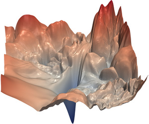
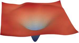
Given a network architecture and its pre-trained parameters, this tool calculates and visualizes the loss surface along random direction(s) near the optimal parameters. The calculation can be done in parallel with multiple GPUs per node, and multiple nodes. The random direction(s) and loss surface values are stored in HDF5 (.h5) files after they are produced.

Setup

Environment: One or more multi-GPU node(s) with the following software/libraries installed:

Pre-trained models: The code accepts pre-trained PyTorch models for the CIFAR-10 dataset. To load the pre-trained model correctly, the model file should contain state_dict, which is saved from the state_dict() method. The default path for pre-trained networks is cifar10/trained_nets. Some of the pre-trained models and plotted figures can be downloaded here:

VGG-9 (349 MB)
ResNet-56 (10 MB)
ResNet-56-noshort (20 MB)
DenseNet-121 (75 MB)

Data preprocessing: The data pre-processing method used for visualization should be consistent with the one used for model training. No data augmentation (random cropping or horizontal flipping) is used in calculating the loss values.

Visualizing 1D loss curve

Creating 1D linear interpolations

The 1D linear interpolation method [1] evaluates the loss values along the direction between two minimizers of the same network loss function. This method has been used to compare the flatness of minimizers trained with different batch sizes [2]. A 1D linear interpolation plot is produced using the plot_surface.py method.

mpirun -n 4 python plot_surface.py --mpi --cuda --model vgg9 --x=-0.5:1.5:401 --dir_type states \
--model_file cifar10/trained_nets/vgg9_sgd_lr=0.1_bs=128_wd=0.0_save_epoch=1/model_300.t7 \
--model_file2 cifar10/trained_nets/vgg9_sgd_lr=0.1_bs=8192_wd=0.0_save_epoch=1/model_300.t7 --plot

--x=-0.5:1.5:401 sets the range and resolution for the plot. The x-coordinates in the plot will run from -0.5 to 1.5 (the minimizers are located at 0 and 1), and the loss value will be evaluated at 401 locations along this line.
--dir_type states indicates the direction contains dimensions for all parameters as well as the statistics of the BN layers (running_mean and running_var). Note that ignoring running_mean and running_var cannot produce correct loss values when plotting two solutions togeather in the same figure.
The two model files contain network parameters describing the two distinct minimizers of the loss function. The plot will interpolate between these two minima.

Producing plots along random normalized directions

A random direction with the same dimension as the model parameters is created and "filter normalized." Then we can sample loss values along this direction.

mpirun -n 4 python plot_surface.py --mpi --cuda --model vgg9 --x=-1:1:51 \
--model_file cifar10/trained_nets/vgg9_sgd_lr=0.1_bs=128_wd=0.0_save_epoch=1/model_300.t7 \
--dir_type weights --xnorm filter --xignore biasbn --plot

--dir_type weights indicates the direction has the same dimensions as the learned parameters, including bias and parameters in the BN layers.
--xnorm filter normalizes the random direction at the filter level. Here, a "filter" refers to the parameters that produce a single feature map. For fully connected layers, a "filter" contains the weights that contribute to a single neuron.
--xignore biasbn ignores the direction corresponding to bias and BN parameters (fill the corresponding entries in the random vector with zeros).

We can also customize the appearance of the 1D plots by calling plot_1D.py once the surface file is available.

Visualizing 2D loss contours

To plot the loss contours, we choose two random directions and normalize them in the same way as the 1D plotting.

mpirun -n 4 python plot_surface.py --mpi --cuda --model resnet56 --x=-1:1:51 --y=-1:1:51 \
--model_file cifar10/trained_nets/resnet56_sgd_lr=0.1_bs=128_wd=0.0005/model_300.t7 \
--dir_type weights --xnorm filter --xignore biasbn --ynorm filter --yignore biasbn  --plot

Once a surface is generated and stored in a .h5 file, we can produce and customize a contour plot using the script plot_2D.py.

python plot_2D.py --surf_file path_to_surf_file --surf_name train_loss

--surf_name specifies the type of surface. The default choice is train_loss,
--vmin and --vmax sets the range of values to be plotted.
--vlevel sets the step of the contours.

Visualizing 3D loss surface

plot_2D.py can make a basic 3D loss surface plot with matplotlib. If you want a more detailed rendering that uses lighting to display details, you can render the loss surface with ParaView.

To do this, you must

Convert the surface .h5 file to a .vtp file.

python h52vtp.py --surf_file path_to_surf_file --surf_name train_loss --zmax  10 --log

This will generate a VTK file containing the loss surface with max value 10 in the log scale.

Open the .vtp file with ParaView. In ParaView, open the .vtp file with the VTK reader. Click the eye icon in the Pipeline Browser to make the figure show up. You can drag the surface around, and change the colors in the Properties window.
If the surface appears extremely skinny and needle-like, you may need to adjust the "transforming" parameters in the left control panel. Enter numbers larger than 1 in the "scale" fields to widen the plot.
Select Save screenshot in the File menu to save the image.

Reference

[1] Ian J Goodfellow, Oriol Vinyals, and Andrew M Saxe. Qualitatively characterizing neural network optimization problems. ICLR, 2015.

[2] Nitish Shirish Keskar, Dheevatsa Mudigere, Jorge Nocedal, Mikhail Smelyanskiy, and Ping Tak Peter Tang. On large-batch training for deep learning: Generalization gap and sharp minima. ICLR, 2017.

Citation

If you find this code useful in your research, please cite:

@inproceedings{visualloss,
  title={Visualizing the Loss Landscape of Neural Nets},
  author={Li, Hao and Xu, Zheng and Taylor, Gavin and Studer, Christoph and Goldstein, Tom},
  booktitle={Neural Information Processing Systems},
  year={2018}
}

sususu1/loss-landscape