The following considerations are presented in this writeup
- Project data sets (training, validation and test) were obtained from the course project GitHub repository.
- The image data set was thoroughly explored and vital statistics were generated, including a label distribution chart. Randomly chosen image samples were also visualized.
- The training dataset was augmented using image transformation techniques. The resulting image set was appended to the original training set. The details of the transformation procedure are presented below.
- LeNet-5 architecture was implemented, trained and tested to two different data set. The first data set was partitioned out of the German dataset.
- Another set was derived based on the Belgain traffic sign database to explore the performance to the trained network. Details discussed in the following sections.
- For the Belgian dataset, the softmax probabilities were studied. About 83% accuracy could be attained.
- Summary of the results will be discussed and presented with reference to the accomanying ipynb HTML submission.
- The loading and summary of datasets is presented in Cell #160 of the ipynb HMTL file.
- The training, validation and testing datasets are loaded from pickle file.
- A summary of the datasets interms of the number of features, labels and array shapes is presented.
- The dataset summary and exploration is performed in Cells #161-#165.
- First, the summary of # of examples in each dataset is presented along with the image data shape (features) and the number of classes (labels).
- The data set is also explored visually uing 3 helper functions (listed in Cell #163).
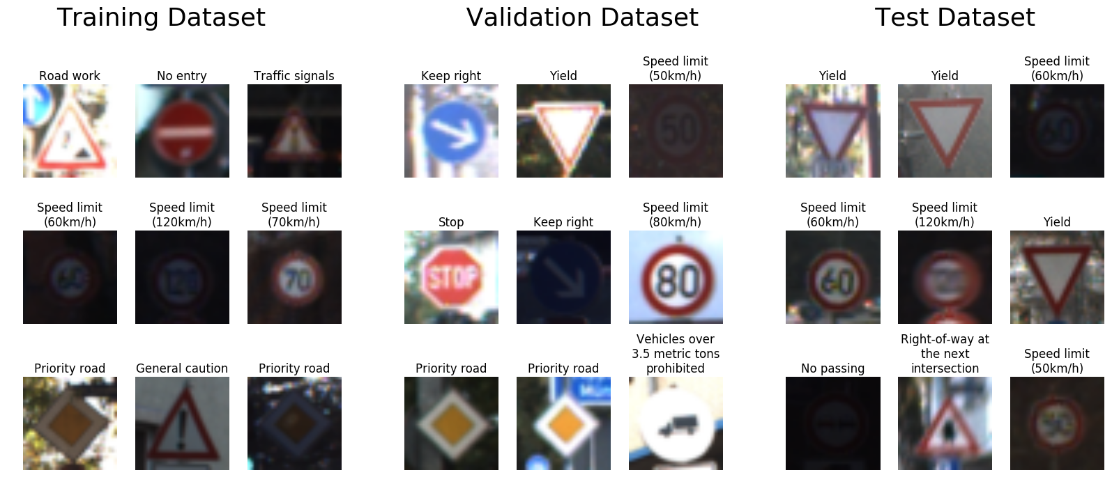
- Nine random images from each dataset are shown, along with the label as title to the figure. This provides a quick summary of the images, and also gives an overview of the image quality of unprocessed images.
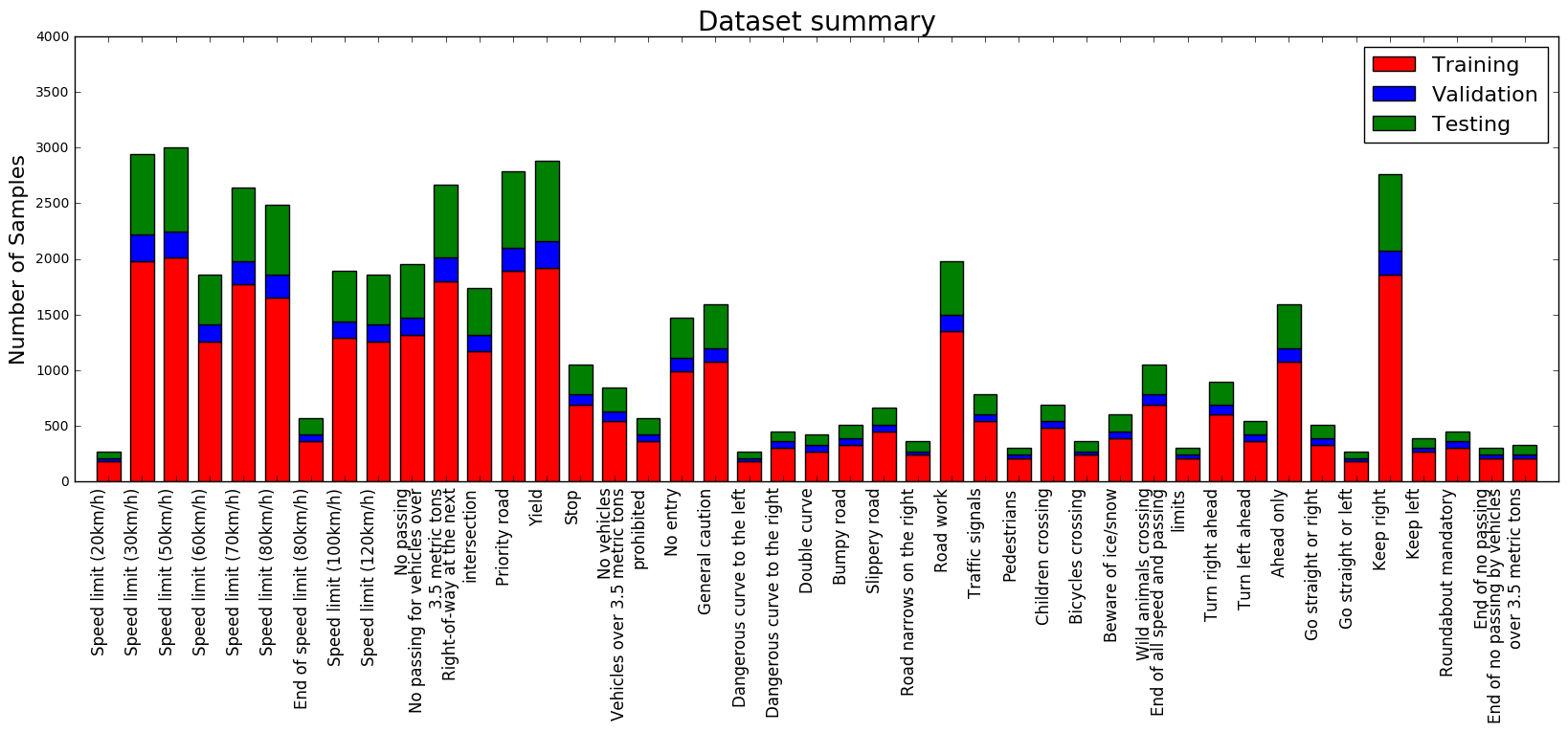
- The distribution of the dataset is also visually explore using a histogram bar chart. The graph showed tha thte speed signs, keep right, yeield, stop and few other labels dominate the training/validation/test datasets.
1. Describe how, and identify where in your code, you preprocessed the image data. What tecniques were chosen and why did you choose these techniques? Consider including images showing the output of each preprocessing technique. Pre-processing refers to techniques such as converting to grayscale, normalization, etc.
An overview of the pre-processing steps and example output is shown in cells #167-171 of the ipynb HTML file. The implementation of the pre-processing steps in the augmentation pipeline is accomplished using two helper functions listed in cell #163.
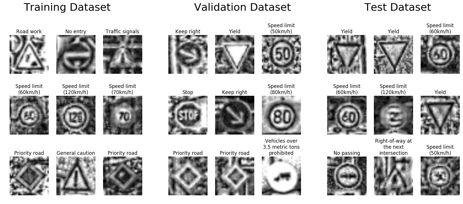
- Function gsnorm_image takes a RGB image as inputs and applies a grayscale fileter using skimage.color.rgb2gray function. Then, it also applies adaptive histogram equalisation to improve the contrast using exposure.equalize_adapthist. Finally, normalization is applied on the grayscale image to change the values to 0.01-0.99 scale using the skimage.exposure.rescale_intensity function. From Figure 1, one can see that the contrast and exposure on some images is extremely poor, which makes it difficult to demarcate the features. The normalized image (shown in Figure 3) clearly demarcates the features.
- Another function augment_image is used to augment the training image dataset. This function applies an affine transform using skimage.transform.AffineTransform function. In other words, rotation, shear and scaling is applied to the image with reference to its center. A great resource on geomtric tranforms can be found here. Note that rotation & shear are critial to the operation and since features are built in raster-form (horizonal / vertical). Simple flip/mirror operation is not enough. In my experience, affine trasnforms give better generalization than flip/mirror during dataset augmentation. Note that care should be taken not to apply too much rotation such that the edges are washed/padded with 0-pixels. This will bias the feature vector and does not add any value.
- In the same augment_image function, Gaussian noise is added to the image to simulate the influence of camera sensor noise and issues during the data acquisition process. This is implemented using skimage.util.random_noise with mode='gaussian' option is used. This is based on the fact that although incident light (photons) arrives at the camera sensor with a Poisson distribution, photon noise is often approximated well using Gaussian distribution when adequate light reaches the sensor, as suggested by the central limit theorem.
2. Describe how, and identify where in your code, you set up training, validation and testing data. How much data was in each set? Explain what techniques were used to split the data into these sets. (OPTIONAL: As described in the "Stand Out Suggestions" part of the rubric, if you generated additional data for training, describe why you decided to generate additional data, how you generated the data, identify where in your code, and provide example images of the additional data)
The code for splitting the data into training and validation sets is contained in the cell #165 of the ipynb HTML file. The final training, validation and test sets sizes are listed below.
- Number of training examples = 34799
- Number of validation examples = 4410
- Number of testing examples = 12630
The examples of the original and augmented images are shown above in Figures 2 & 3.
3. Describe, and identify where in your code, what your final model architecture looks like including model type, layers, layer sizes, connectivity, etc.) Consider including a diagram and/or table describing the final model.
The final model architecture design, training and validation implementation is shown in cell #172-183. The LeNet-5 architecture was adapted from the pervious lab. The implementation is kept similar as before. The structure of the network is listed below.
My final model consisted of the following layers:
| Layer | Description |
|---|---|
| Input | 32x32x1 pre-processed grayscale image |
| Convolution 5x5 | 1x1 stride, VALID padding, outputs 28x28x6 |
| RELU | |
| Max pooling 2x2 | 2x2 stride, outputs 14x14x6 |
| Convolution 5x5 | 1x1 stride, VALID padding, outputs 10x10x16 |
| RELU | |
| Max pooling 2x2 | 2x2 stride, outputs 5x5x16 |
| Flatten layer | Input 5x5x16 and Output 400 |
| Fully connected | Input 400 and Output 120 |
| RELU | |
| Fully connected | Input 120 and Output 84 |
| RELU | |
| Fully connected | Input 84 and Output 43 |
| Softmax | Input 43 and Output 43 labels |
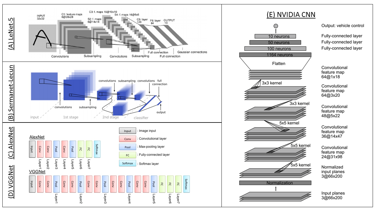
In the present implementation, a derivative of the LeNet-5 architecture (shown in above figure) has been used. There are other convolutional architectures available. These include Sermanet-LeCun, AlexNet, VGGNet, NVIDIA CNN and more. Form the literature, it has been observed that Sermanet-LeCun with drop-out strategy gives the best possible result so far. However, this was not implemented in the presented submission.
Some of the key observation for network model setup are as follows:
- The LeNet-5 network architecture was found satisfactory for the purpose of traffic sign classification.
- Image dataset augmentation by including grayscaled, normalized and affine transformed variants improved accuracy significantly.
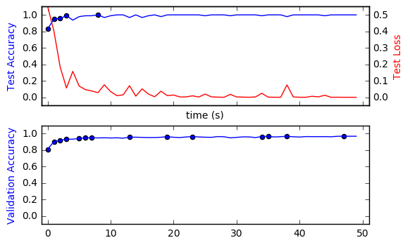
- The training accuracy saturated quickly to 100% within 10 epochs, while the test loss stabilized to low values by 25-30 epochs.
- The validation accuracy also saturated within 10 epochs to a very respectable 97%.
- Overall, with LeNet-5, the accuracy is pretty close typical benchmarks. Further improves upto 99.65% are possible.
Notes for further improvement of the performance (>97%) are as follows:
- Additional steps such as flipping / mirroring can also improve accuracy. However, care has to be taken here not to apply such tranformations to images where there are no folds of symmetry.
- The following architectues are promising and can be explored to further improve accuracy. a. Sermanet-LeCun b. AlexNet c. VGGNet d. NVIDIA CNN
- Implementaiton of drop-out can show some more improvement. More discussion can be found here. I hope to return and improve this project over the course of the next few months.
4. Describe how, and identify where in your code, you trained your model. The discussion can include the type of optimizer, the batch size, number of epochs and any hyperparameters such as learning rate.
The code for training the model is located in the in cell #179 of the ipynb HTML file. To train the model, the following were used.
- Optimizer chosen was AdamOptimizer with a rate of 0.0005
- 50 training EPOCHS with BATCH_SIZE of 128 for the SGD.
- Logits from the network are processed using tf.nn.softmax_cross_entropy_with_logits to determine the SCE and loss function. The optimizer minimized the loss function over the ephocs.
- Following metrics were computed during the course of training. a. Training accuracy and loss b. Validation accuracy.
A history plot of the following metric is shown in the figure below.
In the above plot, it can be seen that the training and validation accuracies quickly reach their peak values within 20 ephocs and remain stable without any subsequent oscillation. The convergence characteristics for the optimizer are good. This is a good indication of correct selection of hyperparameters. The blue dots represent the epoch when the optimizer upgrade to a better training/validation accuracy. The optimizer consistently improved the validation accuracy through the ephocs to reach the peak accuracy of ~97% at epoch 50. Again, this is a sign of good convergence and correct choice of hyperparameters.
5. Describe the approach taken for finding a solution. Include in the discussion the results on the training, validation and test sets and where in the code these were calculated. Your approach may have been an iterative process, in which case, outline the steps you took to get to the final solution and why you chose those steps. Perhaps your solution involved an already well known implementation or architecture. In this case, discuss why you think the architecture is suitable for the current problem.
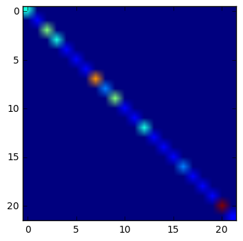
The code for calculating the accuracy of the model is located in the cell # 177. The test dataset from the German traffic sign database was also used and 48 images were randomly selected from the test set to evaluate the test accuracy. This was done after satisfactory results were obtained from the validation set after multiple iterations to tune the hyperparamters. The testing procedure is shown in cell # 219-222. The test accuracy was 100%. The confusion matrix for the test is shown in following figure. Since the test was 100% accurate, there are no off-diagonal elements.
My final model results were:
- Training set accuracy of 100%
- Validation set accuracy of 97%
- Test set accuracy of 100%
If an iterative approach was chosen:
- What was the first architecture that was tried and why was it chosen?
- What were some problems with the initial architecture?
- How was the architecture adjusted and why was it adjusted? Typical adjustments could include choosing a different model architecture, adding or taking away layers (pooling, dropout, convolution, etc), using an activation function or changing the activation function. One common justification for adjusting an architecture would be due to over fitting or under fitting. A high accuracy on the training set but low accuracy on the validation set indicates over fitting; a low accuracy on both sets indicates under fitting.
- Which parameters were tuned? How were they adjusted and why?
- What are some of the important design choices and why were they chosen? For example, why might a convolution layer work well with this problem? How might a dropout layer help with creating a successful model?
If a well known architecture was chosen:
- What architecture was chosen?
- Why did you believe it would be relevant to the traffic sign application?
- How does the final model's accuracy on the training, validation and test set provide evidence that the model is working well?
The first architecture tested was LeCun-5. The implementation from previous lab was adapted. With the intial architecutre, using the color data as features posed significant challenges. The maximum accuracy obtained using the color channels as features was only 89%. It is argued that the traffic signs rarely only differ in color. They may have variation in color, but will also have variation is shape. So, the architeture of the network was adjusted so as to take normalized grayscale images as inputs. After the network was modified, the hyperparameters that were modified were: learning rate, epochs and batch size for SGD. Since the normalized grayscale image improved the inital accuracy, a lower learning rate was explored to improve the accuracy in subsequent epochs. Also, this enabled the use of more number of epochs with a smaller batch size. The resulting network model is extremely efficient in training.
Further improvements can be made to the model. I intend to return to this project to complete implementation of Sermanet-LeCun model with dropout feature. In the literature, it has been shown that this network design is superior to other designs such as AlexNet, VGGNet, NVIDIA CNN, and others. Furthermore, implemetation of the HLSGD method can further improve the optimizer efficiency. State-of-the-art accuracy on the German traffic sign dataset is 99.65%, which is based on the aforementioned combination.
1. Choose five German traffic signs found on the web and provide them in the report. For each image, discuss what quality or qualities might be difficult to classify.
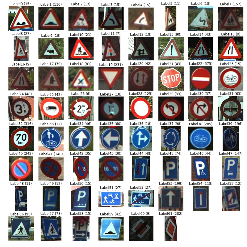
Images were obtained using an academic database post presented on Medium. This is based on the Belgian traffic sign database. 28 images from the following image set were selected for testing purpose.
2. Discuss the model's predictions on these new traffic signs and compare the results to predicting on the test set. Identify where in your code predictions were made. At a minimum, discuss what the predictions were, the accuracy on these new predictions, and compare the accuracy to the accuracy on the test set (OPTIONAL: Discuss the results in more detail as described in the "Stand Out Suggestions" part of the rubric).
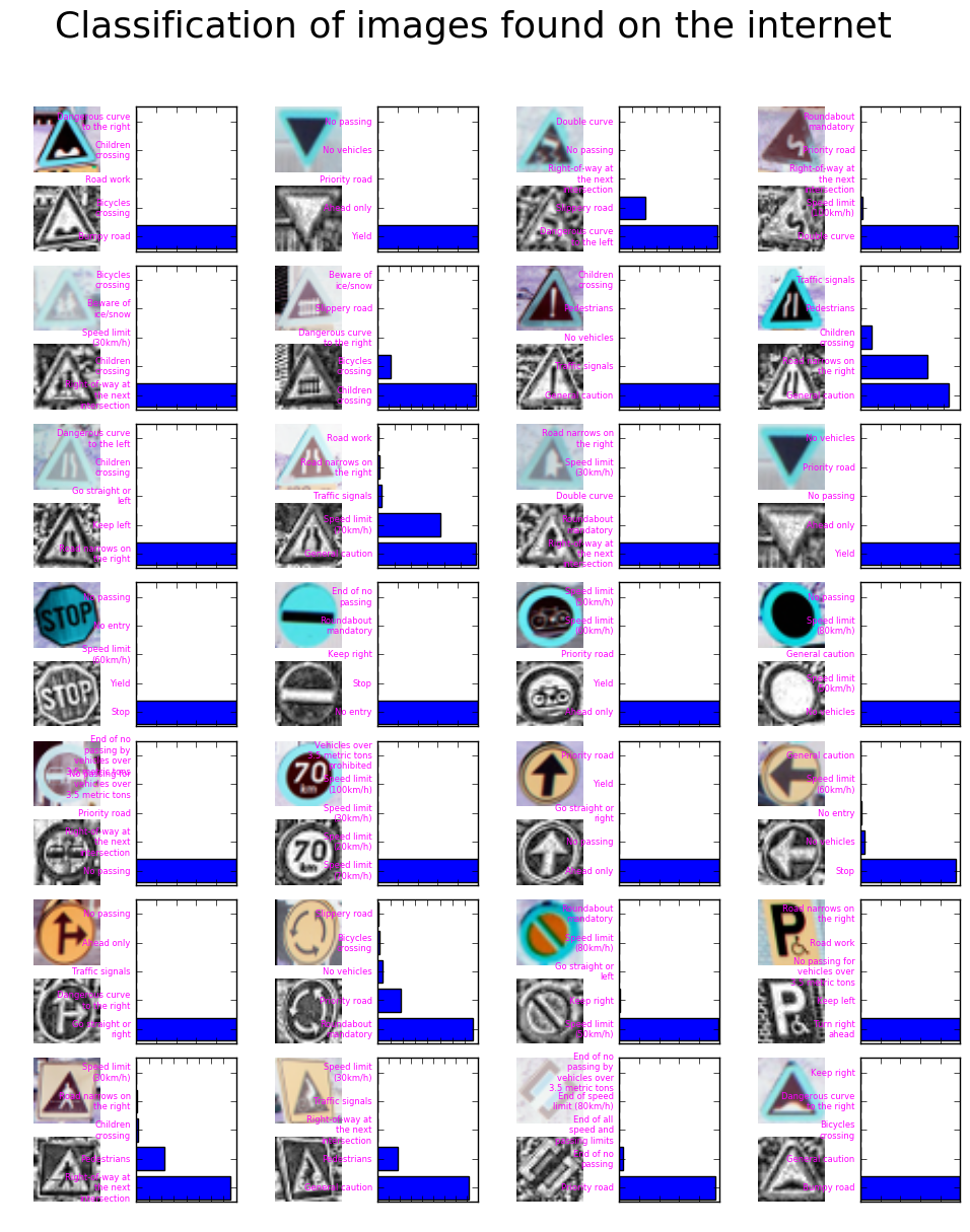
The code for making predictions on my final model is located in cells # 245, 246, 256, 257, 273 & 348 of the ipynb HTML submission file. The following figure gives an overview of the prediction, including the softmax values for the top-5 predictions.
The model was able to correctly guess known traffic signal signs with an accuracy of ~92%. This compares favorably to the accuracy on the test set of 100%.
3. Describe how certain the model is when predicting on each of the five new images by looking at the softmax probabilities for each prediction and identify where in your code softmax probabilities were outputted. Provide the top 5 softmax probabilities for each image along with the sign type of each probability. (OPTIONAL: as described in the "Stand Out Suggestions" part of the rubric, visualizations can also be provided such as bar charts)
The trained network did a decent job with the images obtained from the internet. Since these images are from the Belgian database, there are a few images that were not a part of the training test from the German traffic sign database. The network is able to determine 22 out of 28 images correctly (accuracy ~ 78%). Out of the wrongly identified 6 images, 4 were never presented during the training process (1 railway crossing, 2 cyclists, 1 handicap parking). So, overall the accuracy could be considered 22 out of 24 (92%), which is pretty decent for images from unrelated dataset.
It is also interesting to note that the test set consists of images which have signficantly different aspect ratio compared to tests set (perhaps due to an angle at which the photo was captured). The accuracy of predition seemed to be good, perhpas as a result of the augmented dataset which introduced image histogram normalization and shape distortions. For example, the mandatory roundabout has an aspect ratio different from 1.0 (as was commonly observed in the images from the training set), the trained model was able to label it correctly. Another potential source of error from the custom test set was that some traffic signs were occluded (see the Priority Road sign as an example). However, the network did a good job in classifying it correctly. This is perhaps a one off case (the network got lucky?). A possible robust remedy could be that standard shape based occlusion could be introduced in the augmented databse. Overall, I think the network did a decent job.
