python.ForceBundle

Python / numba Force-directed Edge Bungling for Graph Visualization

Description

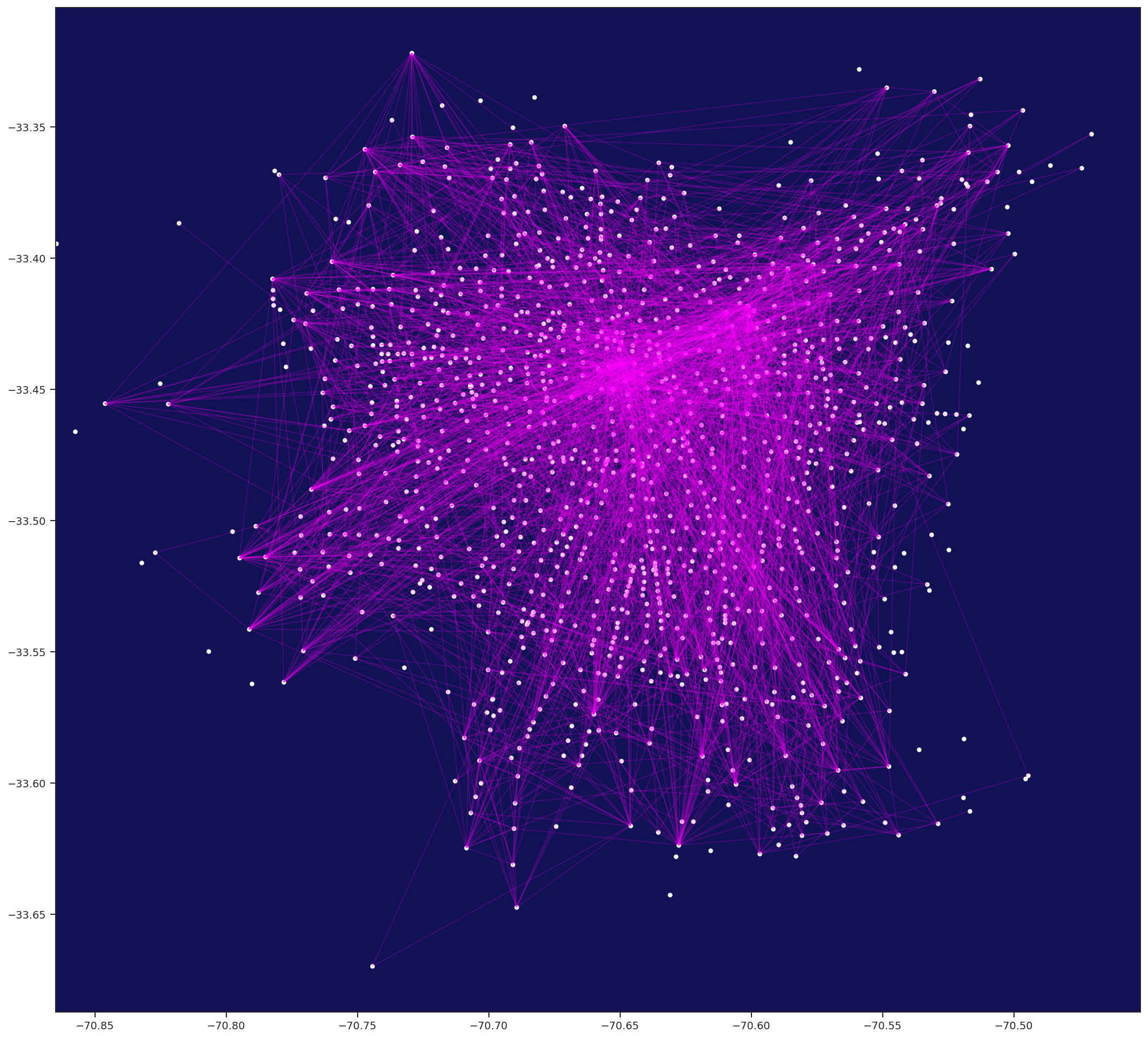
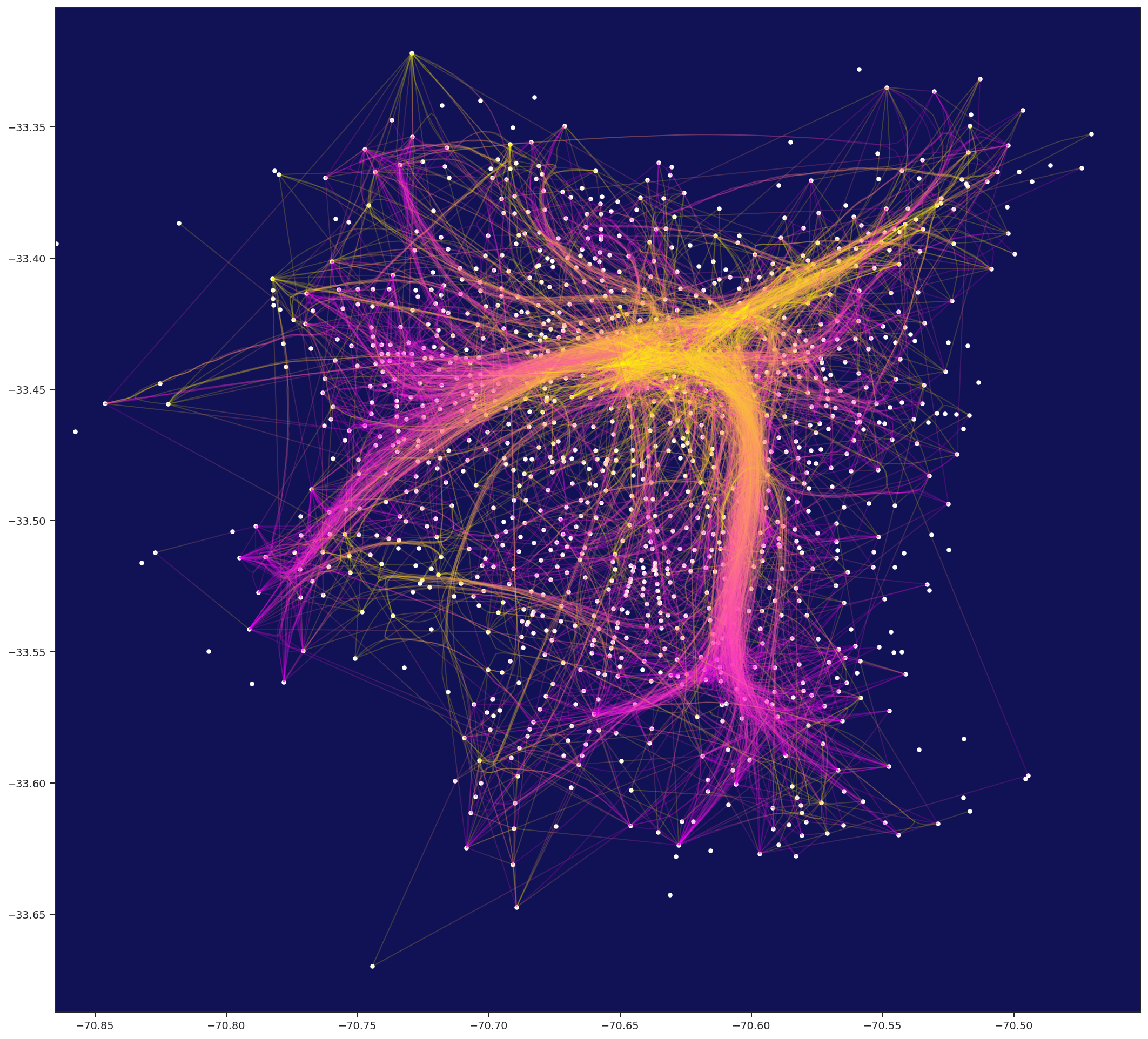
python.ForceBundle is a python implementation of Force-directed Edge Bungling for Graph Visualization, which trough organic bundling of edges, make easy to visualize patterns on otherwise visually clutter diagrams.

Installation

Clone the branch tabita_practica of this repository.

$ git clone https://github.com/tabitaCatalan/python.ForceBundle.git forcebundle
$ cd forcebundle
$ git checkout tabita_practica

Installation options

You should use a virtual environment with Python 3.x. In Option 1 and Option 2, you need to do it before running the pip command. In Option 3 we'll create one using Conda.

Option 1: Minimal requirements

If you only want to use the minimum requirements, just write

$ pip install .

Option 2: Run example notebooks

If you want to learn how to use the package by running the example notebooks, you can write:

$ pip install .[plots]

This will add also jupyter notebooks and some plotting libraries such as matplotlib if they are not available.

Option 3: Run aves example notebook

AVES: Analysis & Visualization -- Education & Support, by Eduardo Graells-Garrido, is a GitHub repository including the dataset of urban movility Encuesta de Origen y Destino de Viajes Santiago 2012. It also has some nice plotting features that we use in aves notebook. AVES is included as a submodule of this repository, but it's not downloaded automatically when you clone this repo. To run this notebook, you can do the following:

Create a environment with the necesary dependencies. If you use Conda, you can use the environment.yml file to create a forcebundle environment with Python 3.8.

conda env create --name forcebundle --file environment.yml

Download AVES source code

# download files from AVES repo
$ git submodule update --init --recursive

Install AVES

# move to AVES directory
$ cd lib/aves

# activate env 
$ conda activate forcebundle

# install AVES in editable mode
pip install -e .

Install forcebundle

# move back to forcebundle directory 
$ cd ../..

# install forcebundle
$ pip install .

Quick start

Download ForcedirectedEdgeBundling.py to you project dir, and use it like this:

# Not really working like this yet
import networkx as nx
import ForcedirectedEdgeBundling as feb

mygraph = nx.read_gml("path.to.file")
input_edges = feb.net2edges(mygraph)
output_lines = feb.forcebundle(input_edges)
bundled_graph = feb.lines2net(output_lines)
bundled_graph.plot()

Check example.ipynb for a full functional example from data to plot.

Parameters Tuning

Fixed Parameters

A certain number of parameters have been fixed to specific optimized values as found through experimentation by the authors. These include the spring constants K (=0.1), which controls the amount of bundling by controling the stiffness of edges. The number of iterations for simulating force interactions I (=60) and the number of cycles of subdivision-force simulation iterations C (=6). Moreover, the initial number of division points P is set to 1 and the rate at which it increases set to 2. The rate of the number of iterations I decreases each cycle is set to 2/3. All these parameters can be changed nonetheless if really needed by using the following methods:

bundling_stiffness ([new bundling stiffness: float value])
iterations([new number of iterations to execute each cycle: int value])
iterations_rate([new decrease rate for iteration number in each cycle: float value])
cycles ([new number of cycles to execute: int value])
subdivision_points_seed([new number subdivision points in first cycle: int value])
subdivision_rate([new rate of subdivision each cycle: float value])

Tuning Parameters For Your Specific Graph

Two parameters are essential for tuning the algorithm to produce usable diagrams for your graph. These are the geometric compatibility score above which pairs of edges should be considered compatible (default is set to 0.6, 60% compatiblity). The value provided should be between 0 and 1. Passing the new value to the compatbility_threshold method will set the new threshold.

The most important parameter is the initial step size used to move the subdivision points after forces have been computed. This depends on both the scale of the graph and the number of edges and nodes contained. Having a step size which is too low will produce node-link like graphs while too high values will over distort edges. This can be set using the step_size function and passing your new step float size value. The default value is set to 0.1.

Contrib & Issues

If you want to contrib, just fork and PR.

If you found a bug, open issue with a minimal, complete, verifiable example.

Debugging

Fixing crashes checklist

Be sure you edges are going trough is_long_enough(edge) or an equibalent (if you using array2edges, it does it for you)
May be the float point:
1. Set FASTMATH=False
2. If still fails try replacing jit spec at Point class from:
```
@jitclass([('x', float32), ('y', float32)])
```
  to:
```
@jitclass([('x', float64), ('y', float64)])
```

Execution flow chart

If you are confused about the execution order of each function, check the execution flow chart.

General debugging advice

Numba function are opaque and big datasets are slow to process without. Mi advice is to attack on both fronts:

Try to slice you edges until you you have a reasonable amount to process without numba , something like:
```
 slide = data[:1000]
 # If doesn't crash then try:
 slide = data[1000:2000] 
```
Go commenting the @jit line on the chain of functions until you find the issue on plain python

beloved js ancestor

This implementation it's a port to numba from un-usably-slow native python implementation which was a port of a d3 js implementation.

I tried to keep structure as close as possible, so bug fixes can be easily ported in both ways.