Cheat sheet for my tutorial SageMath for Beginners: A Quickstart Guide in 60 Minutes | بالعربي
Read the official documentation for installation here
After downloading and installing SageMath, three shortcuts are created on your desktop.
- SageMath console (start typing sageamth commands here)
- SageMath notebook (open jupyter notebook with sage kernel)
- SageMath shell (a normal shell but with sageMath recognized)
To work with SageMath, you can use any of the three shortcuts. I prefer using the SageMath notebook. However i don't recommend launching the SageMath notebook from the shortcut. Instead, To keep things well organized open the SageMath shell and type the following commands:
$ mkdir my-sagemath-new-project
$ cd my-sagemath-new-project
$ sage -n jupyter
This will open a jupyter notebook with the sage kernel. in that directory. Not in the default directory. This is important to organize your work.
SageMath is built on top of Python. So, if you know Python, you already know how to write valid SageMath. Every python code is a valid SageMath code. We can do something that is entirely not related to SageMath and it will still work. For example:
We can make a hello world flask app and it will work.
from flask import Flask
app = Flask(__name__)

@app.route('/')
def hello_world():
    return 'Hello, World!'
This is one of the greatest advantages of SageMath. It is built on top of Python. So, we can use all the features of Python and integrate any functionality we want.
However, SageMath is a mathematical software. So, we will be using it to do mathematical stuff and has some extra features that are not available in Python. These features are the reason why we use SageMath instead of Python.
sage : x = 2
sage : y = 3
sage : x > y
False
sage : x < y
True
sage : x == y
False
sage : x != y
TrueSageMath is a calculator. It can do basic arithmetic operations. For example:
sage : 2 + 2
4
sage : 9 - 3
6
sage : 4 / 2
2
sage : 2 ^ 3 # Not a valid python code
8
sage : 2 ** 3 # Valid python code
8
sage : 2 ^ 2.
4.00000000000000
sage : 2 ^ 2.1
4.28709385014517
sage : 22 // 7 # integer division
3
sage : 22 % 7 # modulus
1Also sageMath comes with a lot of predefined constants. For example:
sage : pi
pi
To show the numerical value of a constant, we can use the n() function. (an optional parameter is digits) For example:
sage : pi.n()
3.14159265358979
sage : pi.n(digits=5)
3.1416
sage : n(pi)
3.14159265358979
sage : e.n()
2.71828182845905
sage : i
Isage : sin(pi)
0
sage : cos(2) # note that is uses radians
cos(2)
sage : cos(2).n()
-0.416146836547142
sage : tan(5).n()
-3.38051500624659
sage : arctan(1)
1/4*pi
sage : arccos(1)
0
sage : arcsin(1).n()
1/2*pisage : exp(1)
e
sage : exp(1).n()
2.71828182845905So lets do something mindblowing
sage : exp(x^2 + log(x))
e^(x^2 + log(x))
sage : exp(x^2 + log(x)).simplify()
x*e^(x^2)
That is actually true
Note that sageMath was able to simplify the expression symbolically. This is one of the greatest features of sageMath. It can simplify expressions symbolically. This is not possible in Python.
Logarithmic functions are also available. For example:
sage : log(2)
log(2)
sage : log(2).n()
0.693147180559945 # default base is e
sage : log(2, e) # log base e
0.693147180559945
sage : ln(2) # ln and log are the same in sage
0.693147180559945
sage : log(128, 2)
7sage : sqrt(2)
sqrt(2)
sage : sqrt(2).n()
1.41421356237310
sage : factorial(5)
120sage : type(2)
<class 'sage.rings.integer.Integer'>
sage : type(2.0)
<class 'sage.rings.real_mpfr.RealLiteral'>
sage : type(2.0 + 3.0*I)
<class 'sage.symbolic.expression.Expression'>
sage: type(pi)
<class 'sage.symbolic.expression.Expression'>
sage: type(pi.n())
<class 'sage.rings.real_mpfr.RealNumber'>
sage : type('hello')
<class 'str'>
sage : type(True)
<class 'bool'>sage: number = 7109
sage: number.is_prime()
True
sage: number.next_prime()
7121
sage: number.previous_prime()
7103
sage: number.divisors()
[1, 7109]
sage: divisors(7642)
[1, 2, 3821, 7642]
sage: number.digits()
[9, 0, 1, 7]
sage: number.ndigits()
4
sage: factor(7642)
2 * 3821
sage: factor(76420) # factorization of a number
2^2 * 5 * 3821
sage: show(sqrt(7))
\sqrt{7}if you are working in jupyter notebook (note the console), the latest command show will output the actual representation
sage: show(sqrt(7))Show some complex expressions
sage : show(integrate(x^2 + 2*x + 1, x))sage : f(x) = x^2 + x - 1
sage : f(x)
x^2 + x - 1
sage : f(2)
5
sage : show(f(x))sage : latex(f(x))
x^{2} + x - 1
sage : solve(f(x) == 0, x)
[x == -1/2*sqrt(5) - 1/2, x == 1/2*sqrt(5) - 1/2]
sage: solve(f(x) == 0, x, solution_dict=True)
[{x: -1/2*sqrt(5) - 1/2}, {x: 1/2*sqrt(5) - 1/2}]
sage : type(f)
<class 'sage.symbolic.expression.Expression'>sage : var('a, b, c')
(a, b, c)
sage : sol = solve(a*x^2 + b*x + c == 0, x); sol
[x == -1/2*(b + sqrt(b^2 - 4*a*c))/a, x == -1/2*(b - sqrt(b^2 - 4*a*c))/a]
sage : show(sol)sage : var('x, y')
(x, y)
sage : solve([x + y == 6, x - y == 4], [x, y])
[[x == 5, y == 1]]
sage : solve([x + y == 5], x, y)
[[x == -r3 + 5, y == r3]]
sage : sol = solve([x^2 + y^2 == 4, x*y == 2], x, y); show(sol)Solving inequalities
sage : solve(x^-2 * x - 1, x)
[[x > 0, x < (1/9)]]sage : f(x) = x^2 + 2*x + 1
sage : show(f.diff())Compute the first derivative
sage : var('u')
u
sage : diff(sin(u), u)
cos(u)
Compute the fourth derivative
sage : diff(sin(x^2), x, 4).show()Compute partial derivatives of
sage : var('x, y')
(x, y)
sage : f = x^2 + 17*y^2
sage : f.diff(x)
2*x
sage : f.diff(y)
34*ysage supports both indefinite and definite integrals
sage : integral(x*sin(x^2), x).show()sage : integral(x/(x^2+1), x, 0, 1).show()When solve fails, you can use find_root to find a root of a numerical solution
sage: theta = var('theta')
sage: solve(cos(theta)==sin(theta), theta) # Nothing interesting here
[sin(theta) == cos(theta)]
sage: find_root(cos(theta)==sin(theta), 0, pi/2) # find a solution in the interval [0, pi/2]
0.7853981633974484
sage: sol = find_root(cos(theta)==sin(theta),0,pi/2); sol
0.7853981633974484
sage: sin(sol)
0.7071067811865476
sage: cos(sol)
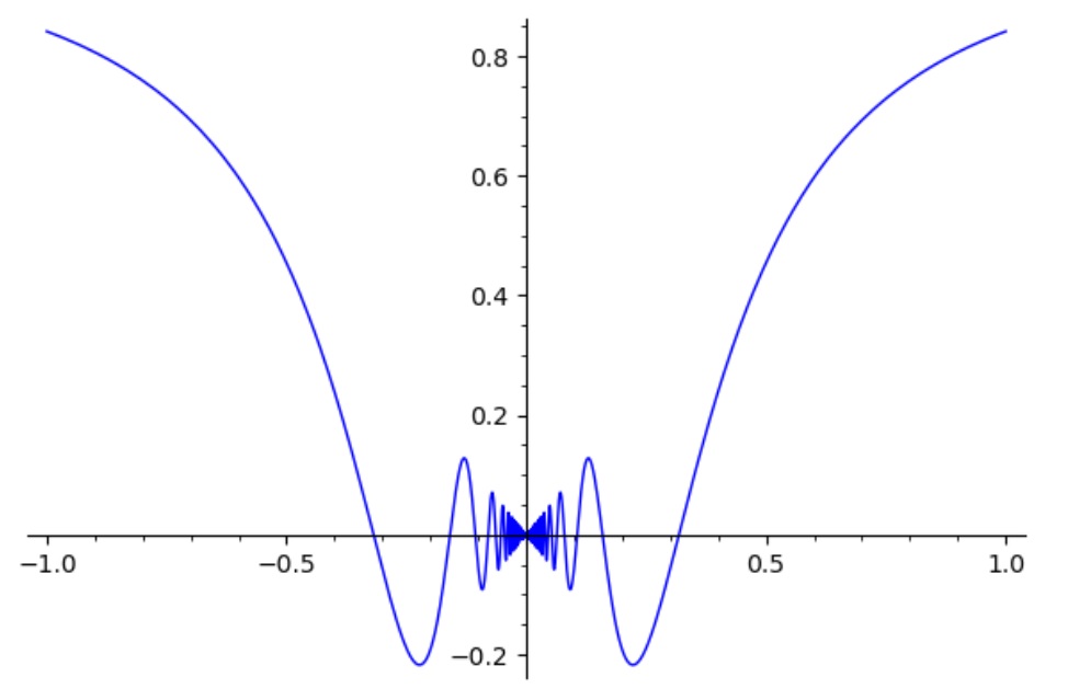
0.7071067811865475sage : f(x) = x*sin(1/x)
sage : f.plot()to plot a function over a specific interval:
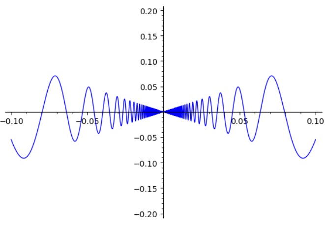
sage : plot(f, (x, -0.1, 0.1), ymin = -0.2, ymax = 0.2)there are countless options to customize the plot, for example:
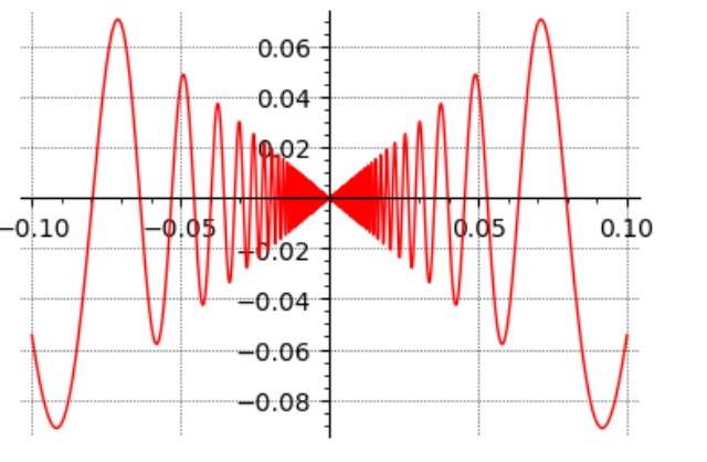
sage : plot(f, (x, -0.1, 0.1), figsize = 4, color = 'red', gridlines = True)More customization:
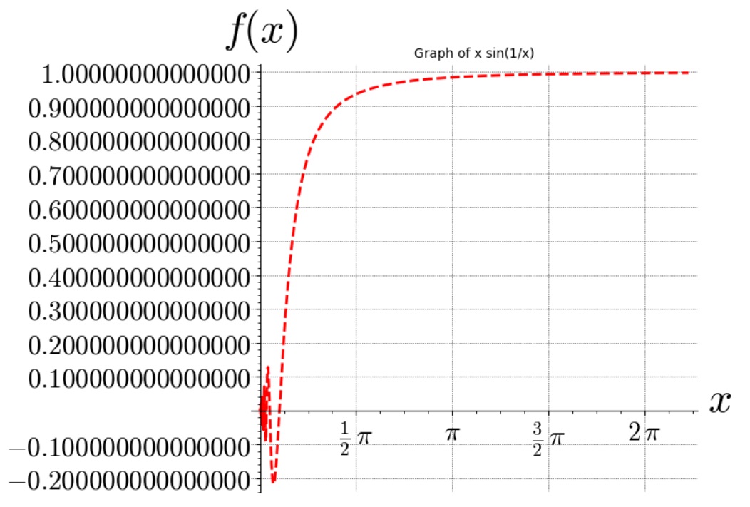
p  = plot(f, (x, 0, 7),
     ymin = -0.2,
     ymax = 1,
     figsize = 8,
     color = 'red',
     gridlines = True,
     thickness = 2,
     linestyle = '--',
     title = 'Graph of x sin(1/x)',
     axes_labels=['$x$', '$f(x)$'],
     ticks = [pi/2, 0.1],
     tick_formatter = [pi/2, 0.1]
     )

p.fontsize(21)
p
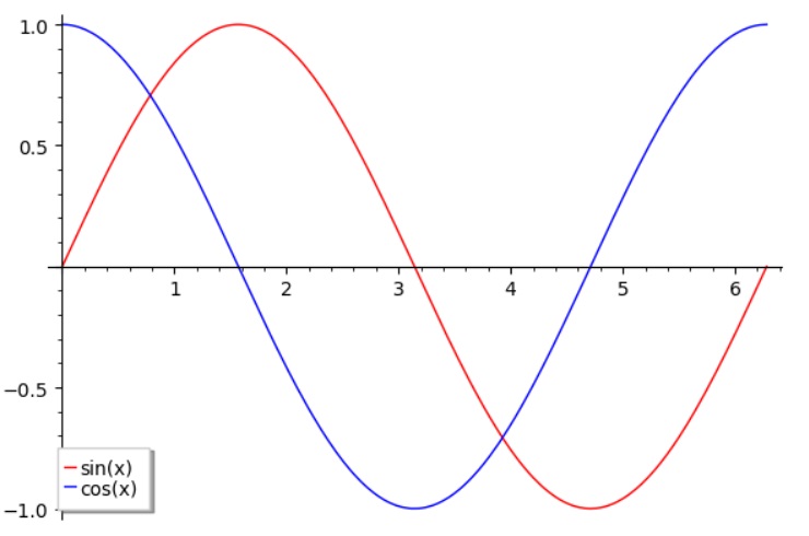
combine multiple plots:
sage : p1 = plot(sin(x), (x, 0, 2*pi), color = 'red', legend_label = 'sin(x)')
sage : p2 = plot(cos(x), (x, 0, 2*pi), color = 'blue', legend_label = 'cos(x)')
sage : p1 + p2
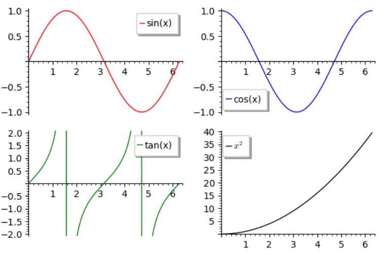
4 plots in one figure: (4 x 4 grid)
sage : p1 = plot(sin(x), (x, 0, 2*pi), color = 'red', legend_label = 'sin(x)')
sage : p2 = plot(cos(x), (x, 0, 2*pi), color = 'blue', legend_label = 'cos(x)')
p3 = plot(tan(x), (x, 0, 2*pi), ymin = -2, ymax = 2, color = 'green', legend_label = 'tan(x)')
sage : p4 = plot(x^2, (x, 0, 2*pi), color = 'black', legend_label = '$x^2$')
sage : graphics_array(((p1,p2), (p3,p4)))
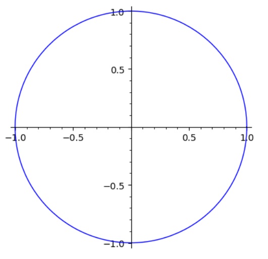
Parametric plots:
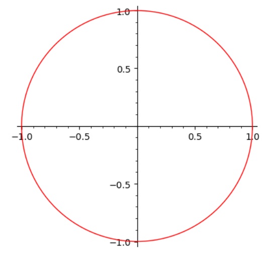
sage : parametric_plot((cos(x), sin(x)), (x, 0, 2*pi))custom shape:
circle((0,0), 1, rgbcolor=(1,0,0)) # center (0,0), radius 1, color redFor more information, see here, you will be amazed by the number of options you can use to customize your plots.
