 Photo by La
La
- R
- renv
renv::restore()
Abalones are an economic and recreational resource that is threatened by a variety of factors which include: pollution, disease, loss of habitat, predation, commercial harvesting, sport fishing and illegal harvesting. Environmental variation and the availability of nutrients affect the growth and maturation rate of abalones. Over the last 20+ years it is estimated the commercial catch of abalone worldwide has declined in the neighborhood of 40%. Abalones are easily over harvested because of slow growth rates and variable reproductive success. Being able to quickly determine the age composition of a regional abalone population would be an important capability. The information so derived could be used to manage harvesting requirements.
The data are derived from an observational study of abalones. The intent of the investigators was to predict the age of abalone from physical measurements thus avoiding the necessity of counting growth rings for aging. Ideally, a growth ring is produced each year of age. Currently, age is determined by drilling the shell and counting the number of shell rings using a microscope. This is a difficult and time consuming process. Ring clarity can be an issue. At the completion of the breeding season sexing abalone can be difficult. Similar difficulties are experienced when trying to determine the sex of immature abalone. The study was not successful. The investigators concluded additional information would be required such as weather patterns and location which affect food availability.
I will analyze the data provided from this study further.
The structure of the data. We can see that there are 1,036 observations (rows) and 8 variables (columns).
## 'data.frame':    1036 obs. of  8 variables:
##  $ SEX   : Factor w/ 3 levels "F","I","M": 2 2 2 2 2 2 2 2 2 2 ...
##  $ LENGTH: num  5.57 3.67 10.08 4.09 6.93 ...
##  $ DIAM  : num  4.09 2.62 7.35 3.15 4.83 ...
##  $ HEIGHT: num  1.26 0.84 2.205 0.945 1.785 ...
##  $ WHOLE : num  11.5 3.5 79.38 4.69 21.19 ...
##  $ SHUCK : num  4.31 1.19 44 2.25 9.88 ...
##  $ RINGS : int  6 4 6 3 6 6 5 6 5 6 ...
##  $ CLASS : Factor w/ 5 levels "A1","A2","A3",..: 1 1 1 1 1 1 1 1 1 1 ...
The basic summary of the data with a table of Class vs Rings.
##  SEX         LENGTH           DIAM            HEIGHT          WHOLE
##  F:326   Min.   : 2.73   Min.   : 1.995   Min.   :0.525   Min.   :  1.625
##  I:329   1st Qu.: 9.45   1st Qu.: 7.350   1st Qu.:2.415   1st Qu.: 56.484
##  M:381   Median :11.45   Median : 8.925   Median :2.940   Median :101.344
##          Mean   :11.08   Mean   : 8.622   Mean   :2.947   Mean   :105.832
##          3rd Qu.:13.02   3rd Qu.:10.185   3rd Qu.:3.570   3rd Qu.:150.319
##          Max.   :16.80   Max.   :13.230   Max.   :4.935   Max.   :315.750
##      SHUCK              RINGS        CLASS        VOLUME
##  Min.   :  0.5625   Min.   : 3.000   A1:108   Min.   :  3.612
##  1st Qu.: 23.3006   1st Qu.: 8.000   A2:236   1st Qu.:163.545
##  Median : 42.5700   Median : 9.000   A3:329   Median :307.363
##  Mean   : 45.4396   Mean   : 9.993   A4:188   Mean   :326.804
##  3rd Qu.: 64.2897   3rd Qu.:11.000   A5:175   3rd Qu.:463.264
##  Max.   :157.0800   Max.   :25.000            Max.   :995.673
##      RATIO
##  Min.   :0.06734
##  1st Qu.:0.12241
##  Median :0.13914
##  Mean   :0.14205
##  3rd Qu.:0.15911
##  Max.   :0.31176

##
##        3   4   5   6   7   8   9  10  11  12  13  14  15  16  17  18  19  20
##   A1   9   8  24  67   0   0   0   0   0   0   0   0   0   0   0   0   0   0
##   A2   0   0   0   0  91 145   0   0   0   0   0   0   0   0   0   0   0   0
##   A3   0   0   0   0   0   0 182 147   0   0   0   0   0   0   0   0   0   0
##   A4   0   0   0   0   0   0   0   0 125  63   0   0   0   0   0   0   0   0
##   A5   0   0   0   0   0   0   0   0   0   0  48  35  27  15  13   8   8   6
##
##       21  22  23  24  25
##   A1   0   0   0   0   0
##   A2   0   0   0   0   0
##   A3   0   0   0   0   0
##   A4   0   0   0   0   0
##   A5   4   1   7   2   1
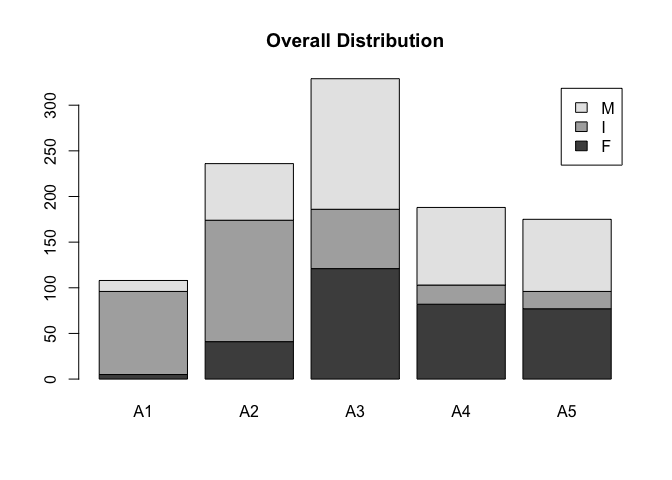
The variables being discussed here is SEX and CLASS. SEX contains male, female, and infant. CLASS are ordered age classification based on RINGS (A1=youngest, and A6= oldest). Overall, the distribution seems like it’s following a normal distribution, but with a slight left skewness. Potential outliers may be abalones that are considered infants in the A4 and A5 groups. Since A4 and A5 are older, their sex should have been identified and it could be an error in the data.
##
##         A1   A2   A3   A4   A5  Sum
##   F      5   41  121   82   77  326
##   I     91  133   65   21   19  329
##   M     12   62  143   85   79  381
##   Sum  108  236  329  188  175 1036
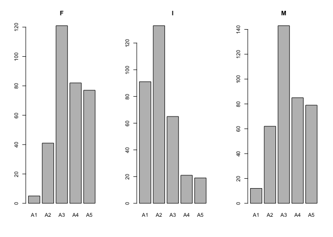
Female and male abalones are left skewed and infant abalones are right skewed in the ordered class. This is most likely because it is harder to identify the sex of younger abalones. The number of infant abalones decrease as the age groups increase because the sex are identified in older groups.
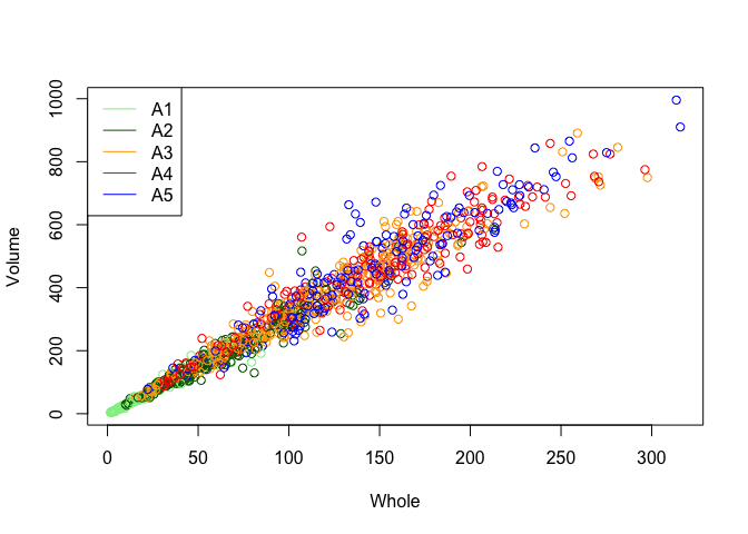
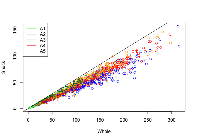
Both plots have a positive correlation to whole. As age groups increase, whole increases and the y variable of volume and shuck increase as well. The first plot has A3-A5 scattered around the middle and top right part of the graph. This behavior seems random without a clear trend. However, for the second plot, we can observe certain trends. The younger groups such as A1-A3 are much closer to the maximum line compared to the older groups such A4-A5. It seems like as abalones age, the ratio of shuck to whole starts to decrease. This is an interesting finding because the first plot is a visualization of volume vs whole. Even though the volume may increase as abalones age, that doesn’t mean the shuck will increase as well.
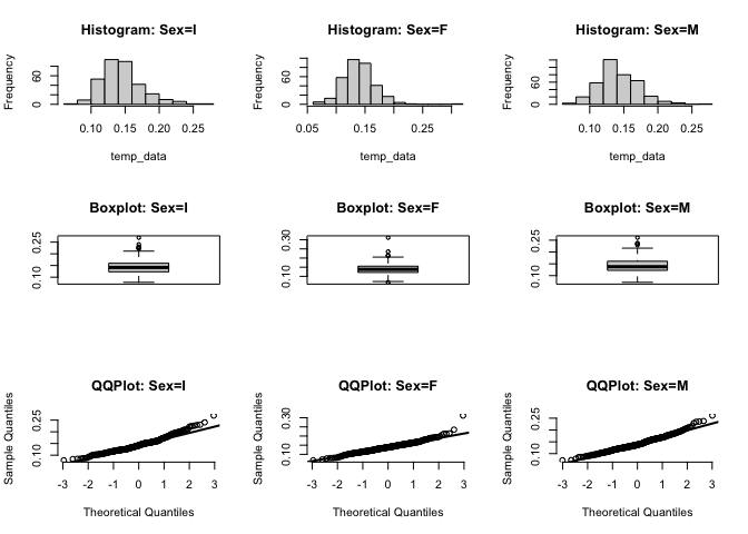
All three sexes are close to a normality. However, all 3 sexes seem to be right skewed as we can observe from the histogram and qqplot. The boxplot shows there are outliers in all 3 sexes above the upper extreme.
| SEX | LENGTH | DIAM | HEIGHT | WHOLE | SHUCK | RINGS | CLASS | VOLUME | RATIO | |
|---|---|---|---|---|---|---|---|---|---|---|
| 3 | I | 10.080 | 7.350 | 2.205 | 79.37500 | 44.00000 | 6 | A1 | 163.364040 | 0.2693371 |
| 37 | I | 4.305 | 3.255 | 0.945 | 6.18750 | 2.93750 | 3 | A1 | 13.242072 | 0.2218308 |
| 42 | I | 2.835 | 2.730 | 0.840 | 3.62500 | 1.56250 | 4 | A1 | 6.501222 | 0.2403394 |
| 58 | I | 6.720 | 4.305 | 1.680 | 22.62500 | 11.00000 | 5 | A1 | 48.601728 | 0.2263294 |
| 67 | I | 5.040 | 3.675 | 0.945 | 9.65625 | 3.93750 | 5 | A1 | 17.503290 | 0.2249577 |
| 89 | I | 3.360 | 2.310 | 0.525 | 2.43750 | 0.93750 | 4 | A1 | 4.074840 | 0.2300704 |
| 105 | I | 6.930 | 4.725 | 1.575 | 23.37500 | 11.81250 | 7 | A2 | 51.572194 | 0.2290478 |
| 200 | I | 9.135 | 6.300 | 2.520 | 74.56250 | 32.37500 | 8 | A2 | 145.027260 | 0.2232339 |
| 350 | F | 7.980 | 6.720 | 2.415 | 80.93750 | 40.37500 | 7 | A2 | 129.505824 | 0.3117620 |
| 379 | F | 15.330 | 11.970 | 3.465 | 252.06250 | 134.89812 | 10 | A3 | 635.827846 | 0.2121614 |
| 420 | F | 11.550 | 7.980 | 3.465 | 150.62500 | 68.55375 | 10 | A3 | 319.365585 | 0.2146560 |
| 421 | F | 13.125 | 10.290 | 2.310 | 142.00000 | 66.47062 | 9 | A3 | 311.979938 | 0.2130606 |
| 458 | F | 11.445 | 8.085 | 3.150 | 139.81250 | 68.49062 | 9 | A3 | 291.478399 | 0.2349767 |
| 586 | F | 12.180 | 9.450 | 4.935 | 133.87500 | 38.25000 | 14 | A5 | 568.023435 | 0.0673388 |
| 746 | M | 13.440 | 10.815 | 1.680 | 130.25000 | 63.73125 | 10 | A3 | 244.194048 | 0.2609861 |
| 754 | M | 10.500 | 7.770 | 3.150 | 132.68750 | 61.13250 | 9 | A3 | 256.992750 | 0.2378764 |
| 803 | M | 10.710 | 8.610 | 3.255 | 160.31250 | 70.41375 | 9 | A3 | 300.153640 | 0.2345924 |
| 810 | M | 12.285 | 9.870 | 3.465 | 176.12500 | 99.00000 | 10 | A3 | 420.141472 | 0.2356349 |
| 852 | M | 11.550 | 8.820 | 3.360 | 167.56250 | 78.27187 | 10 | A3 | 342.286560 | 0.2286735 |
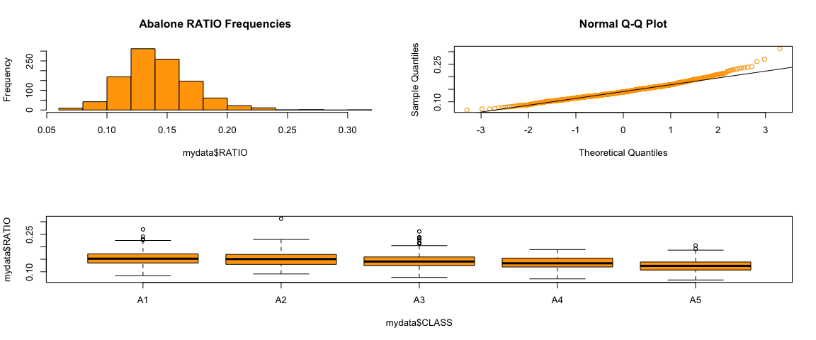
The majority of the outliers have a ratio above 0.22. There was 1 observation that had a ratio of 0.06 which made it as an outlier in the lower extreme. Also, there were no outliers for abalones in the A4 class.
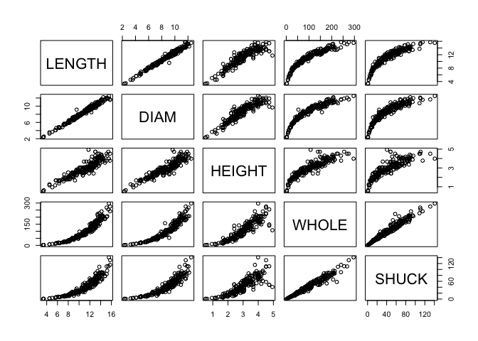
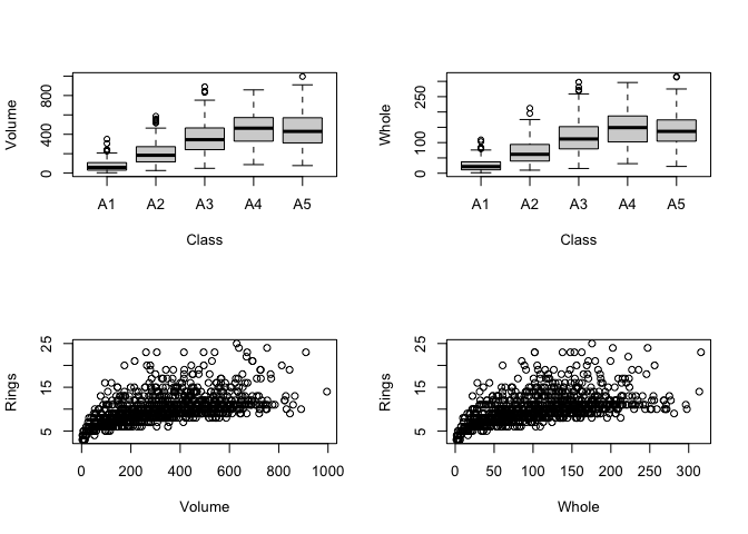
Since there is a positive correlation between the variables, I think it would do fairly well to predict the age. However, as age approaches the A4 & A5 class, it would be difficult to classify because both groups have similar boxplot stats for volume and whole.
| A1 | A2 | A3 | A4 | A5 | |
|---|---|---|---|---|---|
| F | 255.29938 | 276.8573 | 412.6079 | 498.0489 | 486.1525 |
| I | 66.51618 | 160.3200 | 270.7406 | 316.4129 | 318.6930 |
| M | 103.72320 | 245.3857 | 358.1181 | 442.6155 | 440.2074 |
| A1 | A2 | A3 | A4 | A5 | |
|---|---|---|---|---|---|
| F | 38.90000 | 42.50305 | 59.69121 | 69.05161 | 59.17076 |
| I | 10.11332 | 23.41024 | 37.17969 | 39.85369 | 36.47047 |
| M | 16.39583 | 38.33855 | 52.96933 | 61.42726 | 55.02762 |
| A1 | A2 | A3 | A4 | A5 | |
|---|---|---|---|---|---|
| F | 0.1546644 | 0.1554605 | 0.1450304 | 0.1379609 | 0.1233605 |
| I | 0.1569554 | 0.1475600 | 0.1372256 | 0.1244413 | 0.1167649 |
| M | 0.1512698 | 0.1564017 | 0.1462123 | 0.1364881 | 0.1262089 |
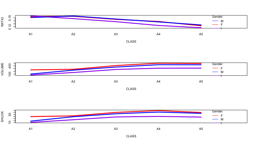
It seems volume and shuck follow a similar trend. As age increases, the volume and shuck increases as well. The females have the highest average volume and shuck in any age group for these 2 variables. However, when it comes to ratio, it follows a different trend. As age increases, the average ratio decreases. Also, the lines intersect frequently. In A1 groups, the infants have the highest ratio. After A2, the female and male keeps intersecting. I wonder why the trend for the ratio are inconsistent compared to volume and shuck. It makes me even wonder if some of the abalones were correctly classified because there are inconsistencies in the ratio.
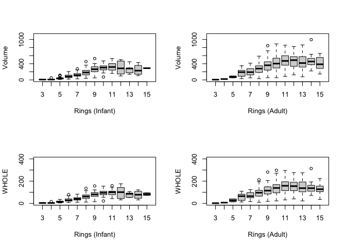
We can suggest that as abalones age, the volume and whole increase. Comparing the infant and adults, we can observe that the adults have more variability as rings increases. The infants have a relatively small variance compared to the adults.
The biggest reason that the original study failed was because it was not possible to completely predict the age of the abalone from the physical measurements. Specifically, the age group of A4-A5 had identical sizes which was difficult to differentiate. For the age groups in early ages such as A1-A3, it may be possibly to predict the age with the physical appearances.
I would inquire if there are certain groups that need to be considered. For example, for studies related to health, age is an extremely important variable. During the COVID pandemic, the Simpson’s paradox became a topic of concern while analyzing the statistics of fatality rate and vaccine effectiveness. I would inquire about any demographic information as possible.
One of the most difficult elements of observational studies is that the sample may not represent the population. For example, even though a study used stratified sampling methods to gather data, the same results may not hold true if the data was collected in an entirely different environment (e.g., country, time of day/year, etc.). With observational studies, correlation can possibly be determined, but not causality. Determining causality would be extremely difficult and it will require domain knowledge and critical thinking.
The structure of the data. We can see that there are 1,036 observations (rows) and 10 variables (columns).
## 'data.frame':    1036 obs. of  10 variables:
##  $ SEX   : Factor w/ 3 levels "F","I","M": 2 2 2 2 2 2 2 2 2 2 ...
##  $ LENGTH: num  5.57 3.67 10.08 4.09 6.93 ...
##  $ DIAM  : num  4.09 2.62 7.35 3.15 4.83 ...
##  $ HEIGHT: num  1.26 0.84 2.205 0.945 1.785 ...
##  $ WHOLE : num  11.5 3.5 79.38 4.69 21.19 ...
##  $ SHUCK : num  4.31 1.19 44 2.25 9.88 ...
##  $ RINGS : int  6 4 6 3 6 6 5 6 5 6 ...
##  $ CLASS : Factor w/ 5 levels "A1","A2","A3",..: 1 1 1 1 1 1 1 1 1 1 ...
##  $ VOLUME: num  28.7 8.1 163.4 12.2 59.7 ...
##  $ RATIO : num  0.15 0.147 0.269 0.185 0.165 ...
## skewness: 0.714705598826372

## kurtosis: 4.66729775944278

## excess kurtosis: 1.66729775944278
## skewness: -0.0939154815619048

## kurtosis: 3.535430948318

## excess kurtosis: 0.535430948318001

##
##  Bartlett test of homogeneity of variances
##
## data:  mydata$RATIO by mydata$CLASS
## Bartlett's K-squared = 21.49, df = 4, p-value = 0.0002531

##
##  Bartlett test of homogeneity of variances
##
## data:  mydata$L_RATIO by mydata$CLASS
## Bartlett's K-squared = 3.1891, df = 4, p-value = 0.5267
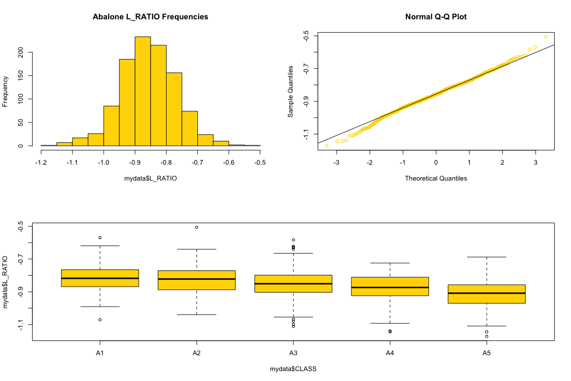
L_RATIO (log ratio) exhibits a better conformance to a normal distribution with homogeneous variances across age. The skewness is close to 0 which indicates it’s a symmetrical distribution. The kurtosis is also close to 3 which indicates it is mesokurtic and resembles a normal distribution peak. We can visually see this with the histogram and qqplot as well. We can also see that the L_RATIO have homogeneous variances across ages with the Barlett test. Since the p-value is much greater than 0.05, we fail to reject the null hypothesis of having identical variances. On the other hand, the RATIO has p-value of 0.0002531 for the Barlett test which indicates that the variances are not homogeneous across ages.
##               Df Sum Sq Mean Sq F value  Pr(>F)
## CLASS          4  1.055 0.26384  38.370 < 2e-16 ***
## SEX            2  0.091 0.04569   6.644 0.00136 **
## CLASS:SEX      8  0.027 0.00334   0.485 0.86709
## Residuals   1021  7.021 0.00688
## ---
## Signif. codes:  0 '***' 0.001 '**' 0.01 '*' 0.05 '.' 0.1 ' ' 1

##               Df Sum Sq Mean Sq F value  Pr(>F)
## CLASS          4  1.055 0.26384  38.524 < 2e-16 ***
## SEX            2  0.091 0.04569   6.671 0.00132 **
## Residuals   1029  7.047 0.00685
## ---
## Signif. codes:  0 '***' 0.001 '**' 0.01 '*' 0.05 '.' 0.1 ' ' 1
While we get statistically significant results with CLASS and SEX independently, that is not the case when we factor CLASS and SEX. We can say there is an interaction effect between these two independent variables. Since both of these variables affects the outcome of L_RATIO, we inevitably get a non-significant result when these two are interacting.
##   Tukey multiple comparisons of means
##     95% family-wise confidence level
##
## Fit: aov(formula = L_RATIO ~ CLASS + SEX, data = mydata)
##
## $CLASS
##              diff         lwr          upr     p adj
## A2-A1 -0.01248831 -0.03876038  0.013783756 0.6919456
## A3-A1 -0.03426008 -0.05933928 -0.009180867 0.0018630
## A4-A1 -0.05863763 -0.08594237 -0.031332896 0.0000001
## A5-A1 -0.09997200 -0.12764430 -0.072299703 0.0000000
## A3-A2 -0.02177176 -0.04106269 -0.002480831 0.0178413
## A4-A2 -0.04614932 -0.06825638 -0.024042262 0.0000002
## A5-A2 -0.08748369 -0.11004316 -0.064924223 0.0000000
## A4-A3 -0.02437756 -0.04505283 -0.003702280 0.0114638
## A5-A3 -0.06571193 -0.08687025 -0.044553605 0.0000000
## A5-A4 -0.04133437 -0.06508845 -0.017580286 0.0000223
##
## $SEX
##             diff          lwr           upr     p adj
## I-F -0.015890329 -0.031069561 -0.0007110968 0.0376673
## M-F  0.002069057 -0.012585555  0.0167236691 0.9412689
## M-I  0.017959386  0.003340824  0.0325779478 0.0111881
We can identify many statistically significant results from different age groups. The only non-significant result we observe was from A2-A1. This indicates that as the abolone’s age group change (besides from A1 to A2), the L_RATIO will change as well. Male and female abalones can be combined into a single category because both have significant differences from infants and we have an extremely high adjusted p-value which suggests there is no difference between male and female.
##
## ADULT     I
##   707   329

## `stat_bin()` using `bins = 30`. Pick better value with `binwidth`.
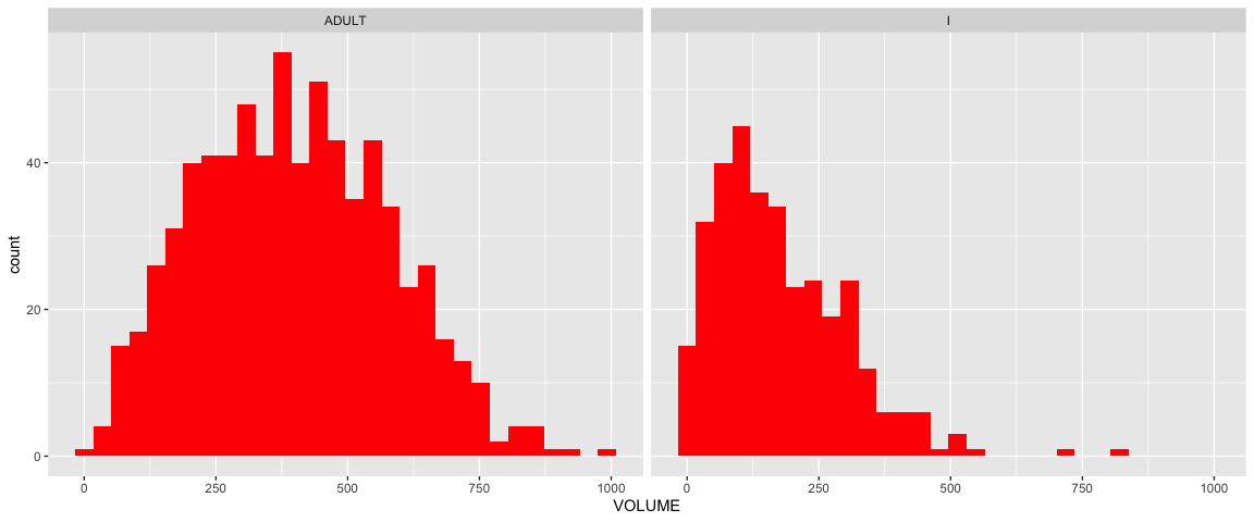
Infants have a right skewed distribution compared to adults. It would be hard to separate infants and adults around the lower volume areas, since there are a lot of overlaps in the two distributions (especially volumes under 300). For larger volumes, it may be easier to separate infants and adults. For volumes over 500, most of the abalones tend to be adults.
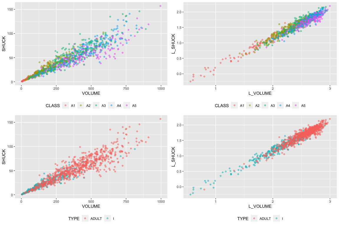
The log-transformation reduces the variability of the relationship between volume and shuck we can make a better distinction between groups. We can see that there is a positive correlation between volume and shuck. For class levels, we can observe that the younger age groups, especially the A1 groups, are separated from the rest. We can observe that in general, when age groups increase, the shuck and volume increase as well. This observation is replicated in the type level. Most of the infants are scattered around the lower end of the volume and shuck. The adults are scattered around the higher end of the volume and shuck.
##
## ADULT     I
##   747   289

##
## Call:
## lm(formula = L_SHUCK ~ L_VOLUME + CLASS + TYPE, data = mydata)
##
## Residuals:
##       Min        1Q    Median        3Q       Max
## -0.270634 -0.054287  0.000159  0.055986  0.309718
##
## Coefficients:
##              Estimate Std. Error t value Pr(>|t|)
## (Intercept) -0.796418   0.021718 -36.672  < 2e-16 ***
## L_VOLUME     0.999303   0.010262  97.377  < 2e-16 ***
## CLASSA2     -0.018005   0.011005  -1.636 0.102124
## CLASSA3     -0.047310   0.012474  -3.793 0.000158 ***
## CLASSA4     -0.075782   0.014056  -5.391 8.67e-08 ***
## CLASSA5     -0.117119   0.014131  -8.288 3.56e-16 ***
## TYPEI       -0.021093   0.007688  -2.744 0.006180 **
## ---
## Signif. codes:  0 '***' 0.001 '**' 0.01 '*' 0.05 '.' 0.1 ' ' 1
##
## Residual standard error: 0.08297 on 1029 degrees of freedom
## Multiple R-squared:  0.9504, Adjusted R-squared:  0.9501
## F-statistic:  3287 on 6 and 1029 DF,  p-value: < 2.2e-16
The summary here shows the reference level of class as A1 and type as adult. The coefficients for classes A2-A5 are the differences associated with A1 and adult. We can imply that the classes A1-A5 are highly correlated variables. When we plotted the data in the scatter plot earlier, it showed positive correlation for volume and shuck for all classes A1-A5 independently. However, when we fit the model and considered all the predictor variables together, we can see that the classes A2-A5 have a negative effect. The coefficients shows that if the data belongs to a class in A2-A5 and holding every other predictors constant, it will have a negative effect when the reference class is A1 and reference type is adult.
Compared to class, type is not as an important predictor for shuck. The coefficient are much smaller compared to most of the other classes. However, it is important to keep in mind that the dependent variable is in log 10 scale. This means that even though it may be a small coefficient, it still can influence the results greatly.
## skewness: -0.0594523446253668

## kurtosis: 3.34330818394132

## excess kurtosis: 0.343308183941319
##
##  Bartlett test of homogeneity of variances
##
## data:  tempdf$residuals by tempdf$CLASS
## Bartlett's K-squared = 3.6882, df = 4, p-value = 0.4498

##
##  Bartlett test of homogeneity of variances
##
## data:  tempdf$residuals by tempdf$TYPE
## Bartlett's K-squared = 0.31156, df = 1, p-value = 0.5767
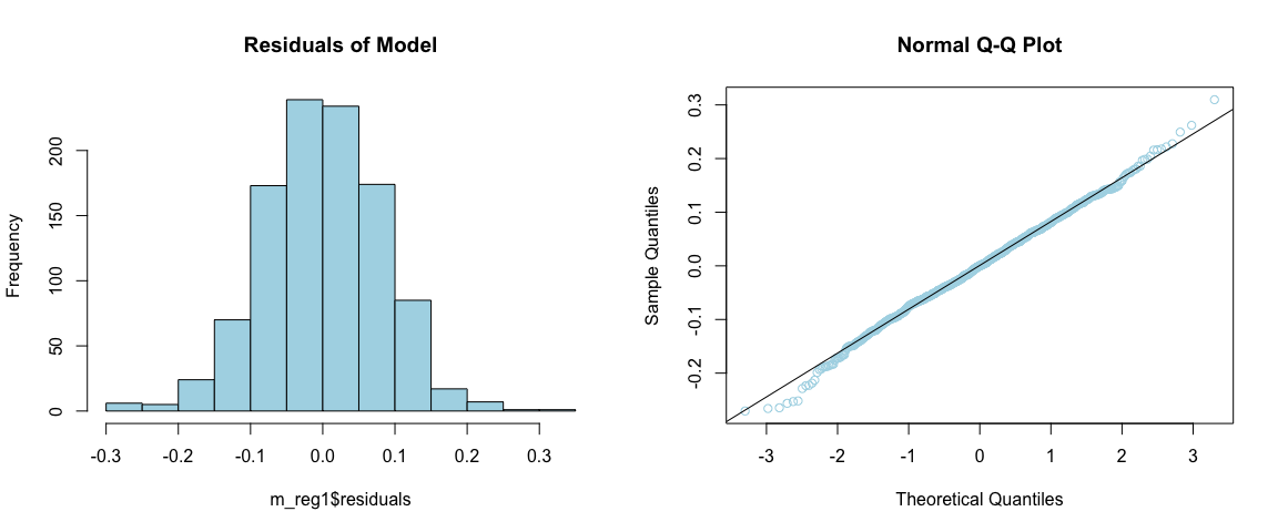
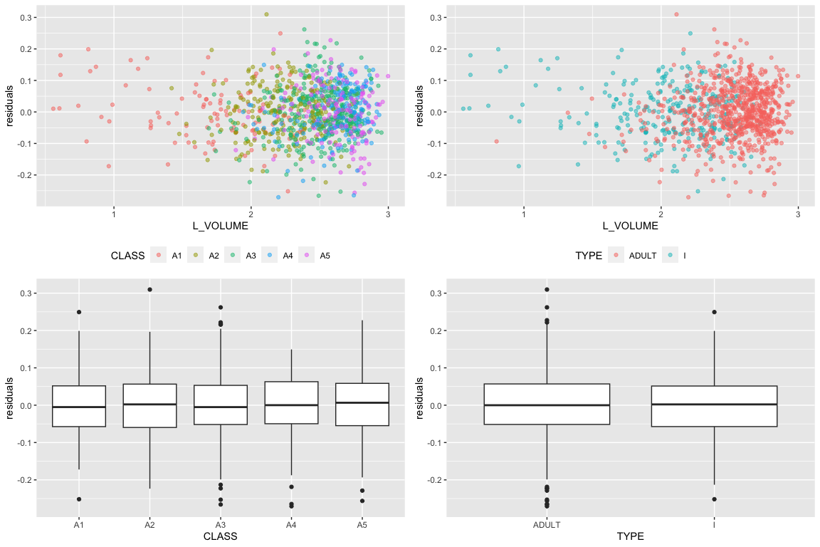
With the above calculations, we checked the assumptions of linear regression. We checked if the residuals were normally distributed and tested the homogeneity of variance of the residuals across classes. Both of these assumptions were met. We can also observe that volume and shuck have a linear relationship from 3(b) and we know each abalones are independent from each other. Therefore, this model indeed fit the dataset and it may be useful for harvesting decisions.
Harvest Strategy:
There is a tradeoff faced in managing abalone harvest. The infant population must be protected since it represents future harvests. On the other hand, the harvest should be designed to be efficient with a yield to justify the effort. This assignment will use VOLUME to form binary decision rules to guide harvesting. If VOLUME is below a “cutoff” (i.e. a specified volume), that individual will not be harvested. If above, it will be harvested. Different rules are possible.The Management needs to make a decision to implement 1 rule that meets the business goal.
## [1] 526.6383

## [1] 0.2476573

## [1] 0

## [1] 133.8214

## [1] 0.4982699

## [1] 0.9330656

## [1] 384.5584

## [1] 0.02422145

## [1] 0.4993307

##
## Attaching package: 'reshape2'

## The following object is masked from 'package:tidyr':
##
##     smiths
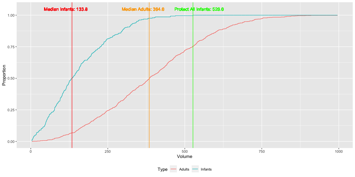
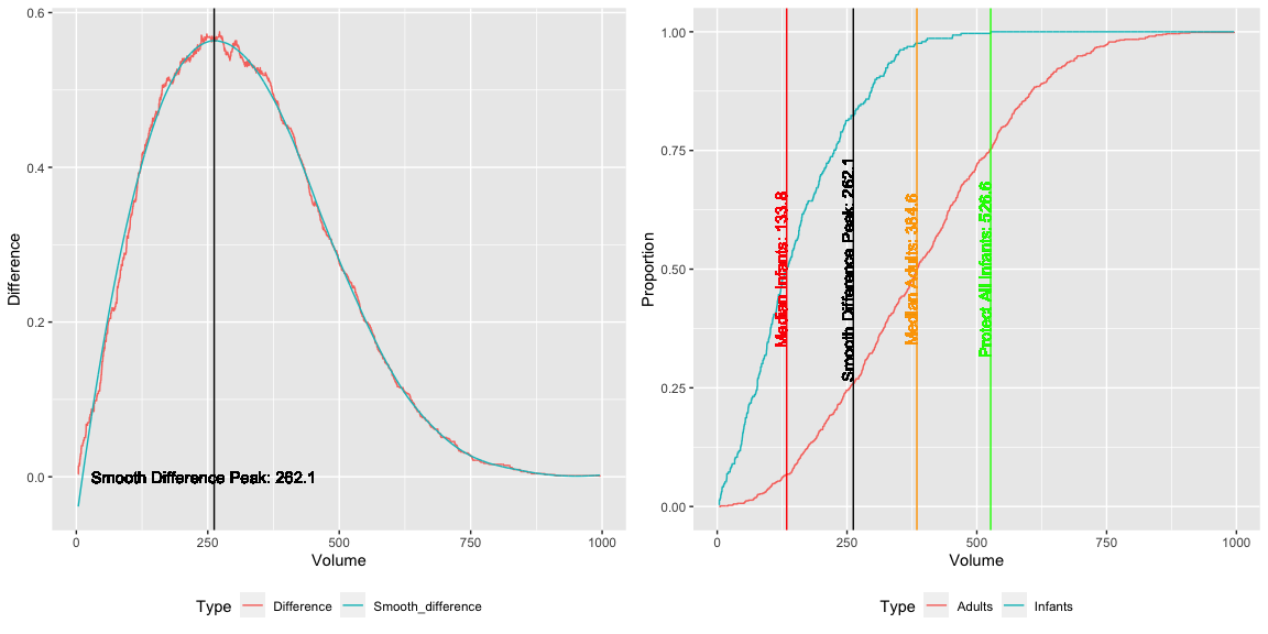
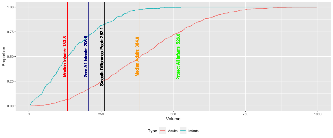
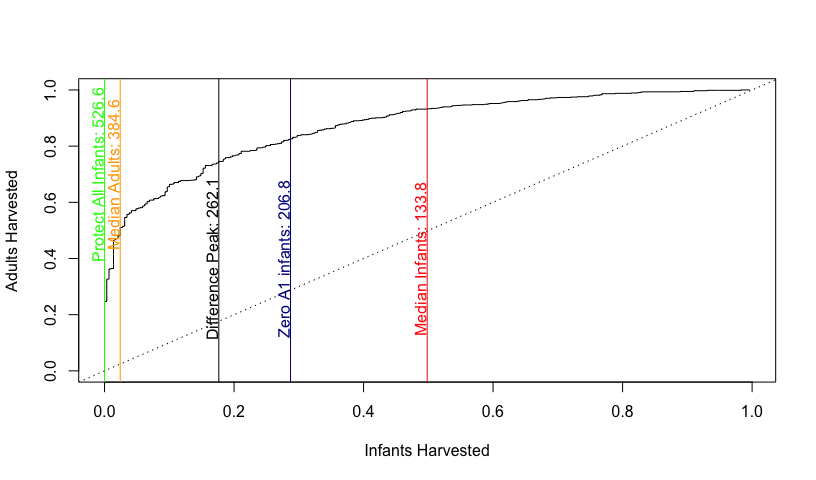
We can clearly observe a difference in median between infants and adults. There will be a trade off of trying to preserve as much infants versus trying to harvest as much adults as possible. Since we want to save as much infants as possible, we don’t want to choose the median infant point as the cut off. This would harvest roughly half of all infants which would have a negative effect on future harvests. Choosing the median adult point as the cut off would be the better option because it would still save roughly 97.6% of all infants while harvesting half of all adults. There needs to be a business decision made based on the choosing the right cut off point for the business.
More harvest strategies:
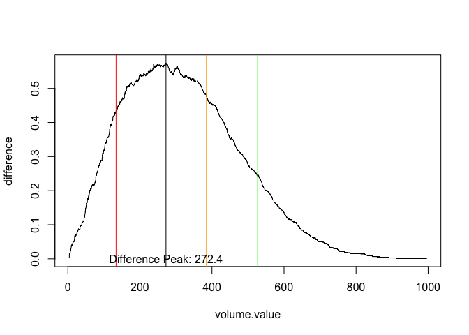
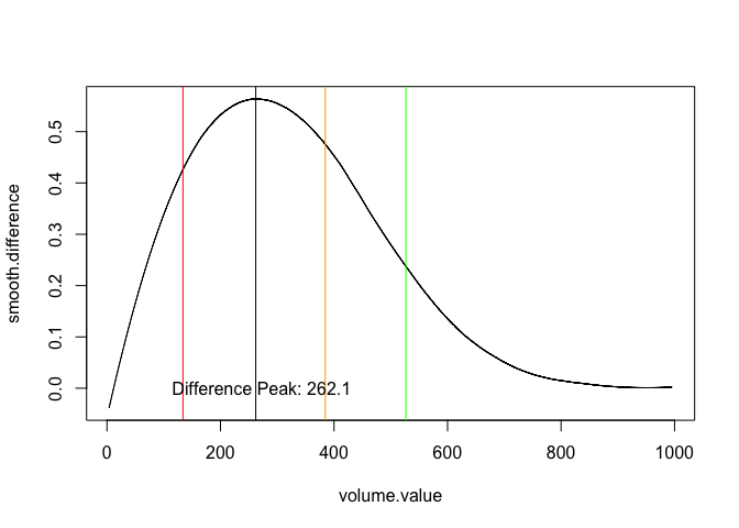
This part will address the determination of a cutoff volume.value corresponding to the observed maximum difference in harvest percentages of adults and infants. In other words, we want to find the volume value such that the vertical distance between the infant curve and the adult curve is maximum. To calculate this result, the vectors of proportions from item (6) must be used. These proportions must be converted from “not harvested” to “harvested” proportions by using (1 - prop.infants) for infants, and (1 - prop.adults) for adults. The reason the proportion for infants drops sooner than adults is that infants are maturing and becoming adults with larger volumes.
## [1] 0.7416332

## [1] 0.7416332

## [1] 0.1764706

## [1] 0.1764706
## [1] 0.2871972

## [1] 0.8259705
## [1] 0.8666894

## [1] 0.246

## [1] 0.1785714

##                      Volume     TPR     FPR totalHarvest
## Protect all infants 526.600   0.246   0.000        0.180
## Median infants      133.800   0.933   0.498        0.813
## Median adults       384.600   0.499   0.024        0.367
## Max difference      262.100   0.742   0.176        0.584
## Zero A1 infants     206.800   0.826   0.287        0.676
There are various thresholds depending on the cutoff volume and there are trade offs. Protect all infants is the most conservative threshold with only harvesting volumes that are equal or greater than 526.8. Because this method is protecting all infants, the FPR is 0, but TPR is limited to 0.246 as well. This will leave out many adult abalones that should have been harvested in order to protect all infants. The median infants, on the other hand, have a very aggressive cutoff volume at 133.8. This method has a high TPR in 0.933, but has a FPR of 0.498. This method harvests roughly half of infant abalones that shouldn’t have been harvested in order to harvest more adults. The median adults, max difference, and zero A1 infants are in between the 2 extreme cutoff points. The business needs to make a decision based on the trade offs of harvesting the abalones now or keeping them for the future.
