Credit risk is the possibility of a loss resulting from a borrower's failure to repay a loan or meet contractual obligations. Traditionally, it refers to the risk that a lender may not receive the owed principal and interest, which results in an interruption of cash flows and increased costs for collection. Excess cash flows may be written to provide additional cover for credit risk. When a lender faces heightened credit risk, it can be mitigated via a higher coupon rate, which provides for greater cash flows.
Although it's impossible to know exactly who will default on obligations, properly assessing and managing credit risk can lessen the severity of a loss. Interest payments from the borrower or issuer of a debt obligation are a lender's or investor's reward for assuming credit risk.
Thus, in order to prevent losses, a proper Credit Risk Management is a must. However, to design it, companies face some challenges that are oftentimes costly and time consuming.
In addition, due to COVID-19, companies will need to strengthen their Credit Risk Management. The Fed has estimated that pandemic-related loan losses for big US banks could reach $700 billion in a worst-case scenario (“double-dip” or W-shaped recession), pushing banks close to their capital minimums.
PS 1: All the references are stated at the end of this README.
PS 2: You can find useful information at section 1 of my notebook.
-
A. Inefficient data management. An inability to access the right data when it’s needed causes problematic delays.
-
B. No groupwide risk modeling framework. Without it, banks can’t generate complex, meaningful risk measures and get a big picture of groupwide risk.
-
C. Constant rework. Analysts can’t change model parameters easily, which results in too much duplication of effort and negatively affects a bank’s efficiency ratio.
-
D. Insufficient risk tools. Without a robust risk solution, banks can’t identify portfolio concentrations or re-grade portfolios often enough to effectively manage risk.
-
E. Cumbersome reporting. Manual, spreadsheet-based reporting processes overburden analysts and IT.
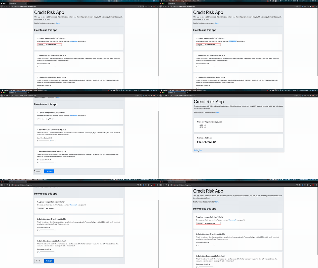
In this project, I managed to address challenges B, D and E by developing a credit risk model that intakes a portfolio of potential customers (.csv file), builds a strategy table and calculates the total expected loss, for example, if we assume that the exposure is the full value of the loan, and the loss given default is 100%. This means that a default on each loan is a loss of the entire amount.
Check it live here: https://credit-risk-bk.herokuapp.com/
OBS: It may take a while to load the app, because I'm using the free tier of Heroku and in this tier app hibernate after 30 min of inactivity.
Key points:
- There are all sorts of ages ranging from 20 to 100+ (outliers were later removed).
- There are all sorts of loan amount, ranging from $500 to $35K.
- Some people allocate high percentage of their income to the loan (max = 83%!).
- By lookin at employment length and credit history, there are people that have been in their early years as employees.
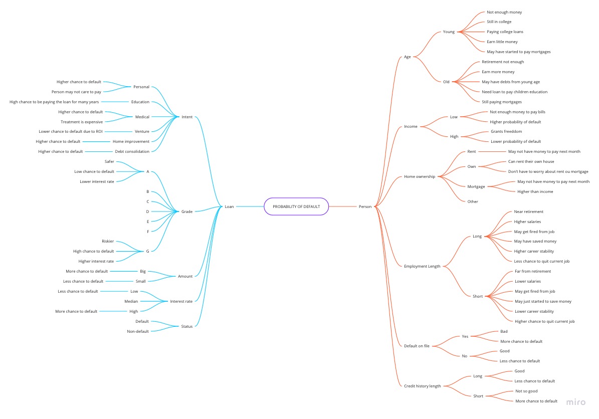
This map to help us to decide which variables we need in order to validate the hypotheses.
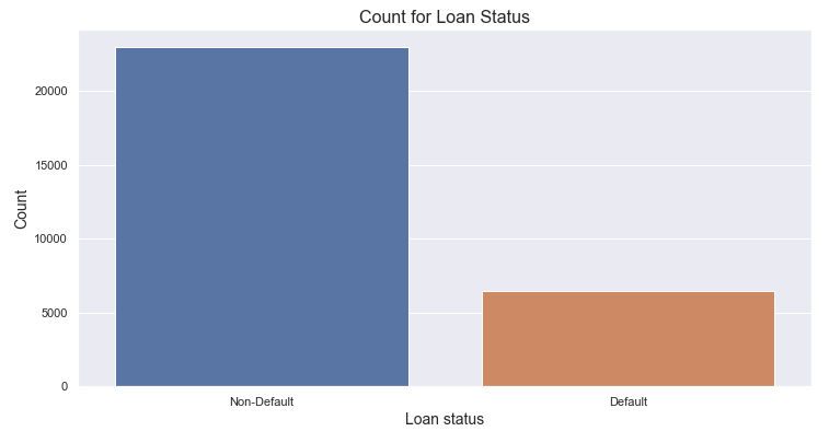
Number of default cases: 6,463 (21.94% of the total loans).
Number of non-defualt cases: 22,996 (78.06% of the total loans).
H3. The median percentage of income to the loan is higher for default than the median for non-default. (TRUE)
As observed, the median of the percentage of income allocated is higher for people who default than for the people who don't.
Thus, the hypothesis is TRUE.
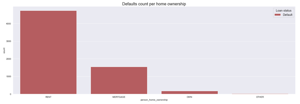
As observed, RENT is the top home ownership type for people who default, not MORTGAGE.
Thus, the hypothesis is FALSE.
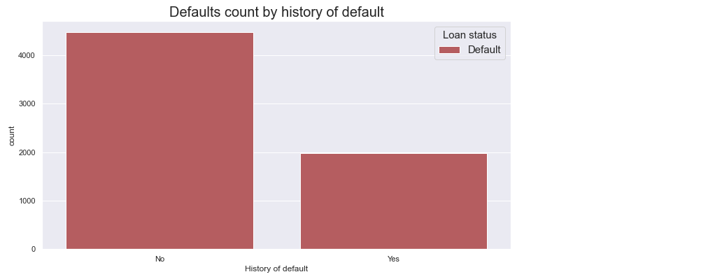
As observed, there are more cases of default for people who don't have history of default.
Thus, the hypothesis is FALSE.
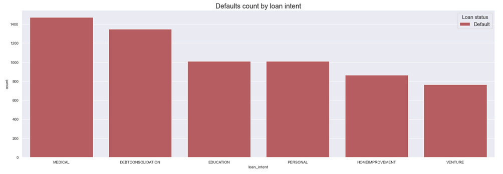
As observed, MEDICAL holds the most number of default cases and VENTURE the least.
Thus, the hypothesis is FALSE.
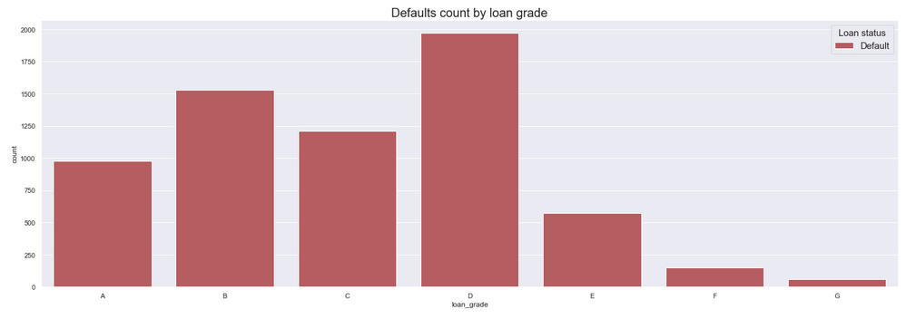
As observed, despite the grade D that is right at the middle grade, the higher the loand grade, the higher is the number of default cases.
Thus, the hypothesis is FALSE.
| ID | Hypothesis | Conclusion |
|---|---|---|
| H1 | There are more defaults for young people | True |
| H2 | People who default have lower income than people who not default | True |
| H3 | The median percentage of income to the loan is higher for default than the median for non-default | True |
| H4 | Mortgage have more cases of default, followed by rent and own | False |
| H5 | The are fewer cases of default for people with long employment length | True |
| H6 | There are more cases of default for people having history of default | False |
| H7 | There are fewer cases of default for people having longer credit history length | True |
| H8 | There are more cases of default for personal than any other intent | False |
| H9 | The least cases of default are for venture | True |
| H10 | The higher the grade, the fewer are the cases of default | False |
| H11 | The loan amount median for default cases is higher than for non-default | True |
| H12 | The interest rate median for default cases is higher than for non-default | True |
Tests were made using different algorithms.
The highlighted cells correspond to the max value at each column.
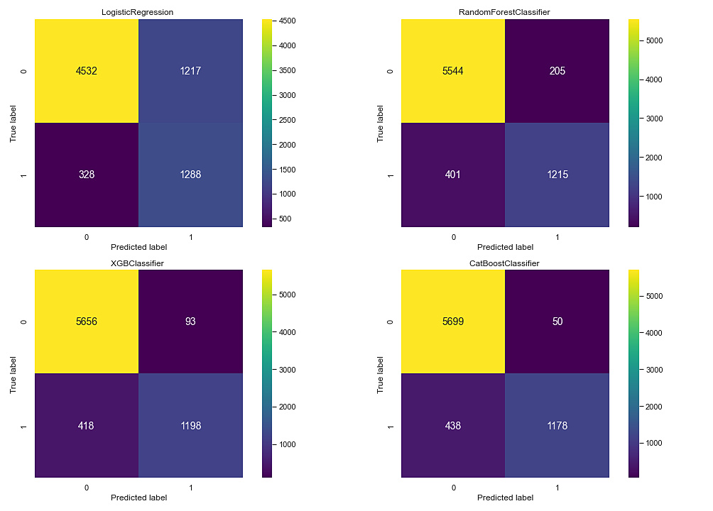
As mentioned before, the CatBoostClassifier satisfies the conditions. But wait, Logistic Regression has the least number of FN, why not choosing it? Yes, it has, but the number of FP is way too high (1217) compared with other algorithms.
As observed, for the context of our project, we are aiming for recall. LogisticRegression presents the highest recall score. However, it's precision score is the lowest. Let's assume we are aiming more for recall and moderate to precision, we could then, take advantage of f1-score, as it's the harmonic average between precision and recall. Thus, the algorithm that satisfies this need is CatBoostClassifier.
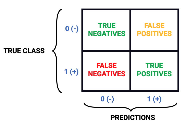
When analyzing the performance metrics for classification machine learning algorithms, we often stumble on the Confusion Matrix.
We need to define which case is the best for the business:
- A) Reduce False Positives (FP) rather than False Negatives (FN).
- B) Reduce False Negatives (FN) rather than False Positives (FP).
In this project, I assumed that the best case for the business was option (B), that is, a default on a loan is worse that not giving a loan to a person.
Thus, it's time to estimate the total expected loss given all our decisions.
- Probabilities of default (PD)
- The loss given default (LGD)
- The loan amount which will be assumed to be the exposure at default (EAD).
Doing the calculations, the total expected loss is $19,596,497.74.
This is the total expected loss for the entire portfolio using the credit risk model developed in this project.
$17.55 million may seem like a lot, but the total expected loss would have been over $29 million without a proper model and $35.4 million without any model at all! Some losses are unavoidable, but this project here might have saved the company about $17.8 million dollars.
The chosen algorithm was the CatBoost Classifier. In addition, I made a performance calibration on it.
These are the metrics obtained from the test set.
| precision | recall | f1-score | roc auc | cohen kappa | accuracy |
|---|---|---|---|---|---|
| 0.9535 | 0.7234 | 0.8227 | 0.9367 | 0.7812 | 0.9316 |
The summary below shows the metrics comparison after running a cross validation score with stratified K-Fold with 10 splits in the full data set.
| Avg Precision | Avg Recall | f1-score | Avg ROC AUC | |
|---|---|---|---|---|
| CatBoost Classifier | 0.8796 (+/- 0.1956) | 0.7190 (+/- 0.1793) | 0.7837 (+/- 0.0976) | 0.9041 (+/- 0.1005) |
| CatBoost Classifier (Tuned HP) | 0.9101 (+/- 0.1554) | 0.7155 (+/- 0.1743) | 0.7947 (+/- 0.0823) | 0.9100 (+/- 0.0847) |
| CatBoost Classifier (Tuned HP + Calibrated) | 0.9625 (+/- 0.0693) | 0.7060 (+/- 0.1808) | 0.8100 (+/- 0.0959) | 0.9094 (+/- 0.0873) |
As observed, although the CatBoost Classifier (Tunned HP) has a higher recall and ROC AUC, its probabilities aren't calibrated, so we're using the CatBoost Classifier (Tuned HP + Calibrated) in our web app because it's worth the trade-off between a little less precision, but a higher calibration quality. In addition, the Tuned HP + Claibrated model has a higher precision and f1-score.
4.1 Address the remaining challenges (A and C).
- https://www.lexingtonlaw.com/credit/length-of-credit-history
- https://www.investopedia.com/terms/c/creditrisk.asp
- https://www.youtube.com/watch?v=bx_LWm6_6tA - The Crisis of Credit Visualized
- https://corporatefinanceinstitute.com/resources/knowledge/finance/credit-risk/
- https://www.sas.com/en_us/insights/risk-management/credit-risk-management.html
- https://www.mckinsey.com/business-functions/risk/our-insights/managing-and-monitoring-credit-risk-after-the-covid-19-pandemic
