[toc]
For this project we are using these primary data sets:
- I94 Immigration Data: This data comes from the US National Tourism and Trade Office. A data dictionary is included in the workspace. This is where the data comes from. There's a sample file so you can take a look at the data in csv format before reading it all in. You do not have to use the entire dataset, just use what you need to accomplish the goal you set at the beginning of the project.
- World Temperature Data: This dataset came from Kaggle. You can read more about it here.
- U.S. City Demographic Data: This data comes from OpenSoft. You can read more about it here.
- Airport Code Table: This is a simple table of airport codes and corresponding cities. It comes from here.
- Additionally there is a SAS Description file that we extract its content to create lookup tables for the all the codes in the immigration data.
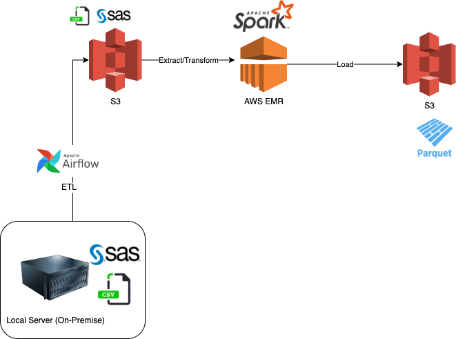
Business wants to start analyzing the data sets, but they are not happy with the current system and want to migrate from their legacy SAS system. They asked to convert the SAS datasets from sas7bdat files to parquet and store them in a Data Lake (S3). The project was driven by the need to migrate to the Cloud (AWS) to make the data accessible to other groups (data science and BI teams). ETL (Extract, Transform and Load) processes were performed to prepare the data.
Goal Migrate legacy system files (SAS Datasets) from on-premise to the cloud and store in a Data Lake (S3). This will later support the Business Intelligence, and Data Science teams in their activities. Business Intelligence team can source the data from the Data Lake and inject into their Data Warehouse.
Business does not have a defined use-case for the data at the moment, but they know for sure they want to migrate away from SAS to another system. The SAS files are large and on a local server (on-premise). They want to make sure the data is formatted and migrated to the cloud for future uses by other departments. This is part of their cloud migration strategy and AWS was selected for this engagement.
The Data Lake will be in Parquet file format hosted on S3 files. The Raw files will also reside in S3 for future archiving and backup.
In this project we will demonstrate the use of:
- Airflow to orchestrate and manage the data pipeline
- AWS EMR for the heavy data processing
- Use Airflow to create the EMR cluster, and then terminate once the processing is complete to save on cost.
The overall project consists of the following steps:
- Gather the SAS files that are part of this project. Currently there are 2.4 GB worth of data files (4 SAS files for the immigration data for April, May, June, and July). There is also a CSV file as well as a data file that contains descriptions which will be used to create lookup tables.
- Migrate the data from on-premise repository (local) to S3 cloud as a staging area
- Create an EMR cluster to process the files.
- Add two new columns: Age-Groups and Age-Categories (using SparkML Bucketizer)
- Cluster the data into 3 clusters based on KMeans clustering algorithm
- Parse the SAS date format for Departure and Arrival dates to a regular Date Format
- Filter the Temperature files and perform additional group-by related transformations
- Push final tables/files into an S3 bucket as Parquet file format
Summary data transformation includes:
- Convert SAS date format into readable date format
- Create Age Group, and Age Category, and Cluster columns
- Temperature data filtered to USA only and averaged by month and city for year > 2003.. Added Year and Month Column
- Create lookup tables for the codes found in the SAS Description file
- Using Airflow to manage the data pipeline and orchestrate the overall flow. Using AWS EMR to do the heavy ETL processes using PySpark. And finally, leverage SparkML to perform Bucketization, and KMeans clustering.
- Leverage the power of Spark for distributed processing to speed up transformation and processing of large SAS datasets (around 13-14M records and 2.6 GB in file sizes).
- Demonstrate how Airflow can play a key role in the corporate strategy for:
- Managing data pipelines
- Data Lineage and Data Quality controls
- Manage AWS resources such as spinning an EMR cluster and then terminating upon job completion.
Overall Architecture
EMR Architecture
├── airflow.sh
├── dags
│   ├── dag.py
│   ├── data
│   │   ├── SAS_data
│   │   │   └── i94_apr16_sub.sas7bdat
│   │   └── csv
│   │       ├── GlobalLandTemperaturesByCity.csv
│   │       ├── airlines.csv
│   │       └── airports.csv
│   ├── jars
│   │   └── spark-sas7bdat-2.0.0-s_2.11.jar
│   └── scripts
│       ├── __init__.py
│       ├── data_values.py
│       └── spark_etl.py
├── docker-compose.yaml
├── logs
└── plugins
- Three main folders which are needed when running Airflow Docker image (see blew instructions). This will mount a docker volume so Airflow running inside the container can access our files from outside.
dags folder- The main file is the
dag.pywhich defines the DAG in Airflow. This file contains the flow, Spark Steps (steps performed once the EMR cluster is running), and EMR configuration (EMR architecture including number of instances, size ..etc) data folderwhich contains two subfolders:csvfolder for CSV files andSAS_datafor our SASsas7bdatfiles.jarfolder which contains any additional JAR files that we need in our EMR Cluster. This can be helpful in cases were we are not able to install needed JAR/packages directly. In most cases installation should work using eitherspark-shelllike thisspark-shell --master local[4] --packages saurfang:spark-sas7bdat:3.0.0-s_2.12or using--packagesinspark-submitlike thisspark-submit --packages saurfang:spark-sas7bdat:2.0.0-s_2.11 spark_etl.pyscriptsfolder contains our mainspark_etl.pyfile which we will execute inside the cluster viaspark-submitcommand. This file contains the entire ELT logic.
- The main file is the
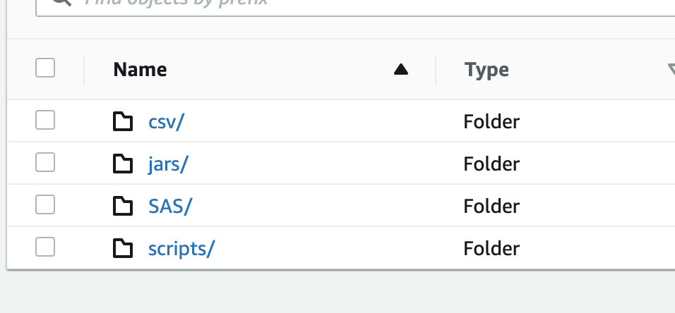
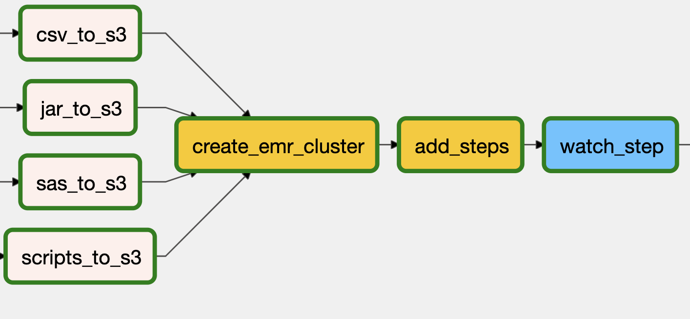
- Migrate all the local data, scripts, and support JAR files from on-premise to S3 in the appropriate folders (image below)
- Create the EMR Cluster as defined in the JOB_FLOW_OVERRIDES (JSON). We will be using several Airflow available operators such as
EmrCreateJobFlowOperator,EmrAddStepsOperator,EmrStepSensor,EmrTerminateJobFlowOperator - Once the cluster is up and running, we will migrate all the need files from S3 to the cluster to be processed inside the cluster. The JAR file will be copied to
/usr/lib/spark/jars/, the data files will all be moved to/sourcefolder. - There are multiple Spark Steps defined. These steps take place inside the cluster. The final output of the ETL though will write the
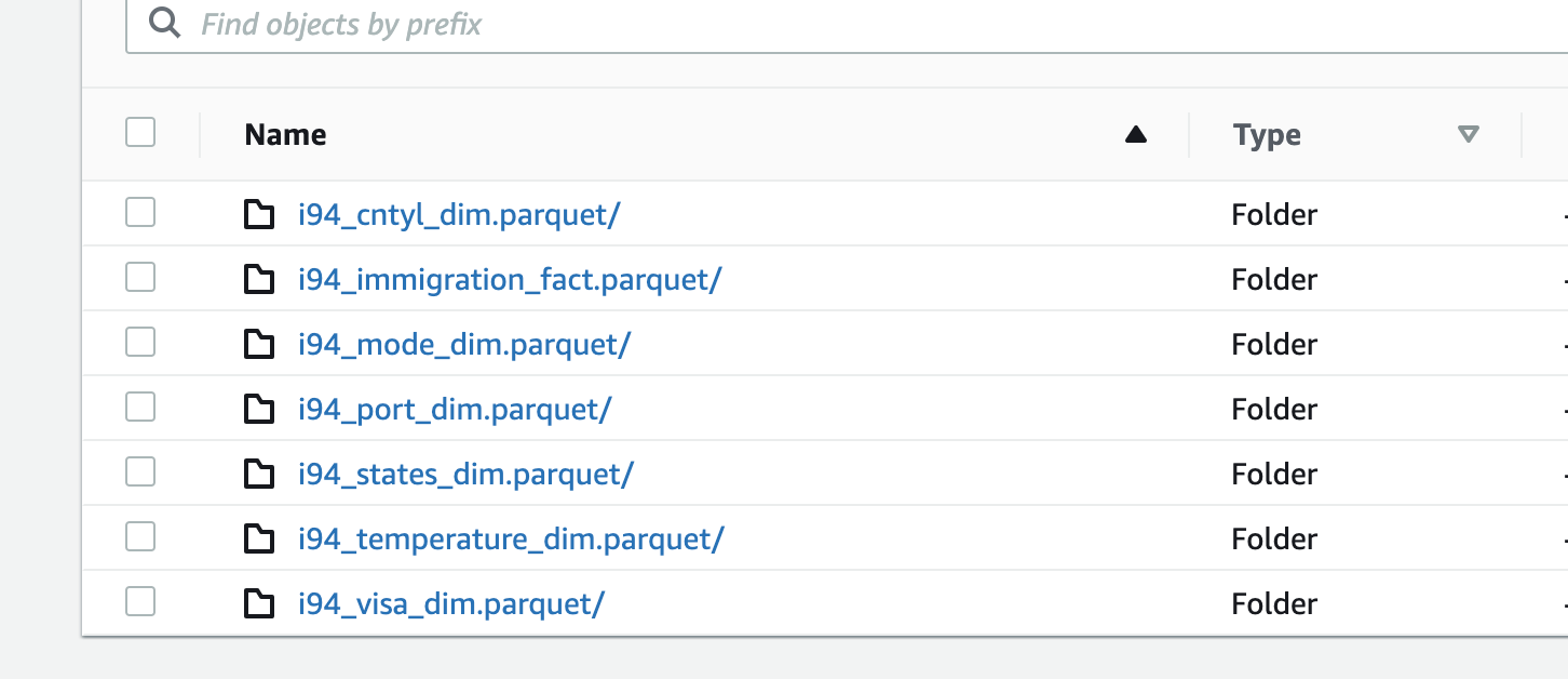
parquetto a local folder namedoutputthat is inside the cluster. The final step, will copy these file from the local cluster to S3 in a folder namedoutputas well - Once copying the files is completed (image below of output folder in S3), the cluster will be terminated.
The DAG below summarized these steps
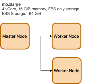
We define the cluster architecture using a key-value structure (like JSON). Here we define a Master Node m5.xlarge and (2) worker nodes also m5.xlarge. The LogUri defined to be on S3.
JOB_FLOW_OVERRIDES = {
    "Name": "Capstone_Project",
    "ReleaseLabel": "emr-5.28.0",
    "Applications": [{"Name": "Hadoop"}, {"Name": "Spark"}],
    "Configurations": [
        {
            "Classification": "spark-env",
            "Configurations": [
                {
                    "Classification": "export",
                    "Properties": {"PYSPARK_PYTHON": "/usr/bin/python3",  "JAVA_HOME": "/usr/lib/jvm/java-1.8.0"},
                },
            ],

        },
    ],
    "Instances": {
        "InstanceGroups": [
            {
                "Name": "Master node",
                "Market": "ON_DEMAND",
                "InstanceRole": "MASTER",
                "InstanceType": "m5.xlarge",
                "InstanceCount": 1,
            },
            {
                "Name": "Core Node",
                "Market": "ON_DEMAND",
                "InstanceRole": "CORE",
                "InstanceType": "m5.xlarge",
                "InstanceCount": 2,
            },
        ],
        "KeepJobFlowAliveWhenNoSteps": True,
        "TerminationProtected": False,
    },
    "JobFlowRole": "EMR_EC2_DefaultRole",
    "ServiceRole": "EMR_DefaultRole",
    "LogUri": "s3://udacity-capstone-2021/job",
    "VisibleToAllUsers": True
}When to use bootstrap actions vs steps in AWS EMR?
Use bootstrap actions to install additional software on an EMR cluster. Use steps to submit work to an EMR cluster, or to process data.
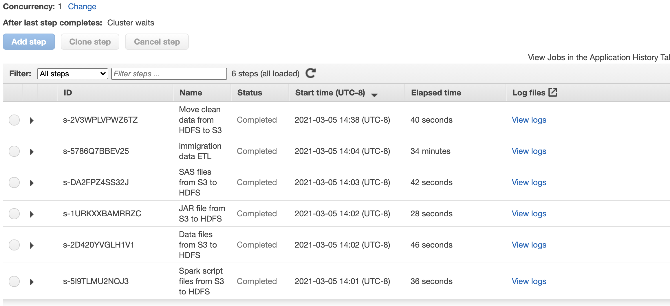
In here will use EMR Steps and define 6 steps:
- Copy script files from S3 source to EMR Cluster under
sourcefolder - Copy data files from S3 source to EMR Cluster under
sourcefolder - Copy JAR files from S3 source to EMR Cluster under
sourcefolder - Copy SAS file from S3 source to EMR Cluster under
/usr/lib/spark/jars/folder - Execute the
spark_etl.pyfile throughspark-submitcommand - Copy the processed data (parquet files) from
outputfolder inside the cluster to S3 bucker inside anoutputfolder
Here is how we define these steps highlights above. This is done using key-value structure (Dictionary) inside a python list.
SPARK_STEPS = [
    {
        "Name": "Spark script files from S3 to HDFS",
        "ActionOnFailure": "CANCEL_AND_WAIT",
        "HadoopJarStep": {
            "Jar": "command-runner.jar",
            "Args": [
                "s3-dist-cp",
                "--src=s3://{{ params.BUCKET_NAME }}/{{ params.s3_script }}",
                "--dest=/source",
            ],
        },
    },
    {
        "Name": "Data files from S3 to HDFS",
        "ActionOnFailure": "CANCEL_AND_WAIT",
        "HadoopJarStep": {
            "Jar": "command-runner.jar",
            "Args": [
                "s3-dist-cp",
                "--src=s3://{{ params.BUCKET_NAME }}/{{ params.s3_data}}",
                "--dest=/source",
            ],
        },
    },
    {
        "Name": "JAR file from S3 to HDFS",
        "ActionOnFailure": "CANCEL_AND_WAIT",
        "HadoopJarStep": {
            "Jar": "command-runner.jar",
            "Args": [
                "s3-dist-cp",
                "--src=s3://{{ params.BUCKET_NAME }}/{{ params.jar_files}}",
                "--dest=/usr/lib/spark/jars/",
            ],
        },
    },
    {
        "Name": "SAS files from S3 to HDFS",
        "ActionOnFailure": "CANCEL_AND_WAIT",
        "HadoopJarStep": {
            "Jar": "command-runner.jar",
            "Args": [
                "s3-dist-cp",
                "--src=s3://{{ params.BUCKET_NAME }}/{{ params.sas_files}}",
                "--dest=/source",
            ],
        },
    },
    {
        "Name": "immigration data ETL",
        "ActionOnFailure": "CANCEL_AND_WAIT",
        "HadoopJarStep": {
            "Jar": "command-runner.jar",
            "Args": [
                "spark-submit",
                "--packages",
                "saurfang:spark-sas7bdat:2.0.0-s_2.11",
                "--deploy-mode",
                "client",
                "s3://udacity-capstone-2021/source_files/scripts/spark_etl.py",
            ],
        },
    },
    {
        "Name": "Move clean data from HDFS to S3",
        "ActionOnFailure": "CANCEL_AND_WAIT",
        "HadoopJarStep": {
            "Jar": "command-runner.jar",
            "Args": [
                "s3-dist-cp",
                "--src=/output",
                "--dest=s3://{{ params.BUCKET_NAME }}/{{ params.s3_clean }}",
            ],
        },
    },
]
There are two main functions in the code.
- process_data which does the heavy ETL process.
- Read the
sas7bdatfile and convert into a Spark data frame - Select relevant columns
- Partition (repartition) to improve performance
- Using SparkML Bucketizer to transform the data frame and add new columns (buckets/bins)
- Read the
- clustering_algorithm
- Data preprocessing including OneHotEncoder, VectorAssembler, and a preprocessing pipeline
- Perform KMeans Clustering (3 clusters)
process_data()
def process_data(spark, file_input, output):
    """
    Primary ETL function for data transformation

    Arguments:
        spark: a spark session
        file_input: data file path
        output: file path to exported data after transformation
    """

    # in this example we will just load one  sas7bdat file given
    df_spark =spark.read.format('com.github.saurfang.sas.spark').load(f'{file_input}/i94_apr16_sub.sas7bdat')

    df = df_spark.select("i94bir",
                    "i94yr",
                    "i94mon",
                    "i94cit",
                    "i94res",
                    "i94port",
                    "arrdate",
                    "i94mode",
                    "i94addr",
                    "depdate",
                    "i94visa",
                    "visapost",
                    "gender",
                    "airline",
                    "fltno",
                    "visatype").dropna(subset=["i94bir"]).repartition(10000)

    ## Create bins/buckets for AgeGroup
    splits = [-float("inf"),12,18,25,35,45,56, 65, 75, float("inf")]
    bucketizer = Bucketizer(splits=splits, inputCol="i94bir", outputCol="AgeGroup")
    df_bucket_1 = bucketizer.setHandleInvalid("keep").transform(df)

    ## Add labels to AgeGroup
    t = {0.0:"Under 12", 1.0: "12-17", 2.0:"18-24", 3.0: "25-34", 4.0: "35-44", 5.0: "45-55", 6.0: "56-64", 7.0: "65-74", 8.0: "75+"}
    udf_foo = udf(lambda x: t[x], StringType())
    df_bucket_1_lbl = df_bucket_1.withColumn("AgeGroupName", udf_foo("AgeGroup"))

    ## Create bins/bucket for AgeCategory
    splits = [-float("inf"), 19, 23, 65, float("inf")]
    bucketizer = Bucketizer(splits=splits, inputCol="i94bir", outputCol="AgeCat")
    df_bucket_2 = bucketizer.setHandleInvalid("keep").transform(df_bucket_1_lbl)

    ## Create labels to AgeCategory
    t = {0.0:"School", 1.0: "College", 2.0:"Professional", 3.0: "Senior"}
    udf_foo = udf(lambda x: t[x], StringType())
    df_bucket_2_lbl = df_bucket_2.withColumn("AgeCatName", udf_foo("AgeCat"))

    date_add_udf = f.udf(date_add_, DateType())

    ## apply to convert arrdate and deprate
    df_bucket_arv = df_bucket_2_lbl.withColumn('actual_arrival_date', date_add_udf('arrdate'))
    df_bucket_dep = df_bucket_arv.withColumn('actual_departure_date', date_add_udf('depdate'))

    # final df_bucket selection
    df_final = df_bucket_dep.select('i94cit',
                            'i94res',
                            'i94port',
                            'i94mode',
                            'i94bir',
                            'i94visa',
                            'i94addr',
                            'gender',
                            'airline',
                            'fltno',
                            'visatype',
                            'AgeGroupName',
                            'AgeCatName',
                            'actual_arrival_date',
                            'actual_departure_date')

    # Convert datasets from python dictionary to PySpark DF
    states_df = spark.sparkContext.parallelize([{"code":k, "name":v} for k,v in states.items()]).toDF()
    i94cntyl_df = spark.sparkContext.parallelize([{"code":k, "name":v} for k,v in i94cntyl.items()]).toDF()
    i94model_df = spark.sparkContext.parallelize([{"code":k, "name":v} for k,v in i94model.items()]).toDF()
    i94prtl_df = spark.sparkContext.parallelize([{"code":k, "name":v} for k,v in i94prtl.items()]).toDF()
    i94visa_df = spark.sparkContext.parallelize([{"code":k, "name":v} for k,v in i94visa.items()]).toDF()

    # GlobalLandTemperatureByCity Data
    fname = f'{file_input}/GlobalLandTemperaturesByCity.csv'
    temp = spark.read.csv(fname, header='true')

    # Aggregate and filter the data
    temp_df = temp.filter(((temp.Country == 'United States' ))& (f.year(f.to_timestamp(temp.dt, 'yyyy-MM-dd')) >= 2003)) \
        .select('AverageTemperature',
                'City',
                'Latitude',
                'Longitude',
                f.month(f.to_timestamp(temp.dt, 'yyyy-MM-dd')).alias('month'))\
        .groupBy('month', 'City').agg(f.avg('AverageTemperature').alias('AvgTemp'), f.max('Latitude').alias('Latitude'), f.max('Longitude').alias('Longitude'))

    # time table
    time_table = df_final.select(
                    f.col('actual_arrival_date').alias('date'),
                    f.year('actual_arrival_date').alias('year'),
                    f.month('actual_arrival_date').alias('month'),
                    f.dayofmonth('actual_arrival_date').alias('dayofmonth'),
                    f.weekofyear('actual_arrival_date').alias('weekofyear')
                        )

    # Write out the data sets
    df_final.repartition("airline", "i94mode").write.partitionBy("airline", "i94mode").mode("overwrite").parquet(f"{output}/i94_immigration_fact.parquet", mode="overwrite")

    states_df.write.parquet(f"{output}/i94_states_dim.parquet", mode="overwrite")
    i94cntyl_df.write.parquet(f"{output}/i94_cntyl_dim.parquet", mode="overwrite")
    i94model_df.write.parquet(f"{output}/i94_mode_dim.parquet", mode="overwrite")
    i94prtl_df.write.parquet(f"{output}/i94_port_dim.parquet", mode="overwrite")
    i94visa_df.write.parquet(f"{output}/i94_visa_dim.parquet", mode="overwrite")
    temp_df.write.parquet(f"{output}/i94_temperature_dim.parquet", mode="overwrite")
clustering_algorithm
def clustering_algorithm(spark, input_data):
    """
    Function to perform KMeans clustering. This function take the Spark session, and input dataframe,
    then performs OneHotEncoding and additional preprocessing steps to finally add a `cluster` columns.
    """
    print("==Clustering Algorithm Started==")
    # Cluster Data Set
    from pyspark.ml.feature import VectorAssembler, OneHotEncoderEstimator, OneHotEncoder, OneHotEncoderModel, StringIndexer
    from pyspark.ml import Pipeline
    from pyspark.ml.clustering import KMeans


    cols = ["i94addr", "visatype", "i94port", "gender", "airline", "AgeGroupName", "AgeCatName"]
    othercols = ['i94cit', 'i94res', 'i94mode', 'i94bir', 'i94visa']

    indexers = [
        StringIndexer(inputCol=c, outputCol="{0}_indexed".format(c))
        for c in cols
    ]

    encoders = [ OneHotEncoder(inputCol=indexer.getOutputCol(),
                    outputCol="{0}_encoded".format(indexer.getOutputCol()))
                    for indexer in indexers ]

    assembler = VectorAssembler(inputCols=[encoder.getOutputCol() for encoder in encoders]
                                    +othercols , outputCol="features")

    ff = input_data.select("i94addr",
                        "visatype",
                        "i94port",
                        "gender",
                        "airline",
                        "AgeGroupName",
                        "AgeCatName",
                        "i94cit",
                        "i94res",
                        "i94mode",
                        "i94bir",
                        "i94visa").dropna().dropDuplicates().repartition(1000)

    preprocess = Pipeline(stages=indexers + encoders + [assembler]).fit(ff)

    data = preprocess.transform(ff)

    kmeans = KMeans(k=3, seed=1)  # 3 clusters
    model = kmeans.fit(data.select('features'))
    transformed = model.transform(data)
    cluster_df = transformed.select("i94addr", "visatype", "i94port", "gender", "airline",
        'i94cit', 'i94res', 'i94mode', 'i94bir', 'i94visa', 'AgeGroupName', 'AgeCatName', f.col("prediction").alias("cluster")
    )

cluster_df.repartition("cluster").write.partitionBy("cluster").mode("overwrite").parquet("i94_data/i94_immigration_cluster.parquet")To deploy Airflow on Docker Compose, you should fetch docker-compose.yaml.
curl -LfO 'https://airflow.apache.org/docs/apache-airflow/2.0.1/docker-compose.yaml'This file contains several service definitions:
airflow-scheduler- The scheduler monitors all tasks and DAGs, then triggers the task instances once their dependencies are complete.airflow-webserver- The webserver available athttp://localhost:8080.airflow-worker- The worker that executes the tasks given by the scheduler.airflow-init- The initialization service.flower- The flower app for monitoring the environment. It is available athttp://localhost:8080.postgres- The database.redis- The redis - broker that forwards messages from scheduler to worker.
All these services allow you to run Airflow with CeleryExecutor. For more information, see Basic Airflow architecture.
Some directories in the container are mounted, which means that their contents are synchronized between your computer and the container.
./dags- you can put your DAG files here../logs- contains logs from task execution and scheduler../plugins- you can put your custom plugins here.
Before starting Airflow for the first time, You need to prepare your environment, i.e. create the necessary files, directories and initialize the database.
On Linux, the mounted volumes in container use the native Linux filesystem user/group permissions, so you have to make sure the container and host computer have matching file permissions.
mkdir ./dags ./logs ./plugins
echo -e "AIRFLOW_UID=$(id -u)\nAIRFLOW_GID=0" > .env
On all operating system, you need to run database migrations and create the first user account. To do it, run.
docker-compose up airflow-initAfter initialization is complete, you should see a message like below.
airflow-init_1       | Upgrades done
airflow-init_1       | Admin user airflow created
airflow-init_1       | 2.0.1
start_airflow-init_1 exited with code 0
The account created has the login airflow and the password airflow.
Now you can start all services:
docker-compose upIn the second terminal you can check the condition of the containers and make sure that no containers are in unhealthy condition:
$ docker ps
CONTAINER ID   IMAGE                  COMMAND                  CREATED          STATUS                    PORTS                              NAMES
247ebe6cf87a   apache/airflow:2.0.1   "/usr/bin/dumb-init …"   3 minutes ago    Up 3 minutes              8080/tcp                           compose_airflow-worker_1
ed9b09fc84b1   apache/airflow:2.0.1   "/usr/bin/dumb-init …"   3 minutes ago    Up 3 minutes              8080/tcp                           compose_airflow-scheduler_1
65ac1da2c219   apache/airflow:2.0.1   "/usr/bin/dumb-init …"   3 minutes ago    Up 3 minutes (healthy)    0.0.0.0:5555->5555/tcp, 8080/tcp   compose_flower_1
7cb1fb603a98   apache/airflow:2.0.1   "/usr/bin/dumb-init …"   3 minutes ago    Up 3 minutes (healthy)    0.0.0.0:8080->8080/tcp             compose_airflow-webserver_1
74f3bbe506eb   postgres:13            "docker-entrypoint.s…"   18 minutes ago   Up 17 minutes (healthy)   5432/tcp                           compose_postgres_1
0bd6576d23cb redis:latest "docker-entrypoint.s…" 10 hours ago Up 17 minutes (healthy) 0.0.0.0:6379->6379/tcp compose_redis_1After starting Airflow, you can interact with it in 3 ways;
- by running CLI commands.
- via a browser using the web interface.
- using the REST API.
You can also run CLI commands, but you have to do it in one of the defined airflow-* services. For example, to run airflow info, run the following command:
docker-compose run airflow-worker airflow infoIf you have Linux or Mac OS, you can make your work easier and download a optional wrapper scripts that will allow you to run commands with a simpler command.
curl -LfO 'https://airflow.apache.org/docs/apache-airflow/2.0.1/airflow.sh'
chmod +x airflow.sh
Now you can run commands easier.
./airflow.sh infoYou can also use bash as parameter to enter interactive bash shell in the container or python to enter python container.
./airflow.sh bash./airflow.sh pythonTo stop and delete containers, delete volumes with database data and download images, run:
docker-compose down --volumes --rmi all- When doing a lot of transformations, such as
.dropna()or.dropDuplicates()as an example, it is a good idea to check the number of partitions as things may change and can cause issues later on. This can be done usinggetNumPartitions()
df_final.rdd.getNumPartitions()And adjusting the partition can be done simply using repartition
df_final.repartition(1000)- Repartition creates same size partitions and can speed up overall execution and process.
repartitionpartition data in memory whilepartitionBycreates on Disk before write.- You can combined
repartitionandpartitionBylike in this example
df_final.repartition("airline", "i94mode").write.partitionBy("airline", "i94mode").mode("overwrite").parquet(f"{output}/i94_immigration_fact.parquet", mode="overwrite")
- The data was increased by 100x.
- The pipelines would be run on a daily basis by 7 am every day.
- The database needed to be accessed by 100+ people.
The data was increased by 100x
Leveraging AWS EMR is a scalable option. To handle larger data, increasing the size of the cluster, and number of nodes would allow Spark to handle larger amount of data.
Also, batch processing would speed up the overall process of migrating the data. We can partition the data in Spark to improve performance.
The pipelines would be run on a daily basis by 7 am every day.
Airflow makes it easy to setup a schedule, form daily, weekly, monthly ..etc.
dag = DAG("emr_dag",
          default_args=default_args,
          description="Load and transform with Airflow and AWS EMR-Spark",
          schedule_interval="@daily"
          )
If we want this to occur daily at 7 am then we can use cron style like this 0 7 * * *
dag = DAG("emr_dag",
          default_args=default_args,
          description="Load and transform with Airflow and AWS EMR-Spark",
          schedule_interval="0 7 * * *"
          )
The database needed to be accessed by 100+ people.
Right now the data is in S3, which can scale and handle man concurrent users without issues. AWS makes it easy to scale this way through replication and portioning behind the scene. Similarly, if the data was stored in AWS RDS, or Redshift, can handle simultaneous client connections and requests.
For example RDS
| DB engine | Parameter | Allowed values | Default value | Description |
|---|---|---|---|---|
| MariaDB and MySQL | max_connections |
1–100000 | {DBInstanceClassMemory/12582880} | Number of simultaneous client connections allowed |
| Oracle | processes |
80–20000 | LEAST({DBInstanceClassMemory/9868951}, 20000) | User processes |
sessions |
100–65535 | – | User and system sessions | |
| PostgreSQL | max_connections |
6–8388607 | LEAST({DBInstanceClassMemory/9531392}, 5000) | Maximum number of concurrent connections |
| SQL Server | Maximum number of concurrent connections | 0–32767 | 0 (unlimited) | Maximum number of concurrent connections |
Similarly, AWS Redshift has a set of limits and quota which can be accessed here. For an increase on those limits, there is a request form https://console.aws.amazon.com/support/home?#/case/create?issueType=service-limit-increase&limitType=service-code-redshift

