slopes
The goal of slopes is to enable fast, accurate and user friendly calculation longitudinal steepness of linear features such as roads and rivers, based on commonly available input datasets such as road geometries and digital elevation model (DEM) datasets.
Installation
Install the development version from GitHub with:
# install.packages("remotes")
remotes::install_github("itsleeds/slopes")
Usage
Load the package in the usual way:
library(slopes)We will also load the sf library:
library(sf)
#> Linking to GEOS 3.8.0, GDAL 3.0.4, PROJ 7.0.0
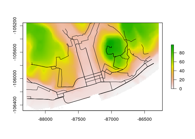
The minimum data requirements for using the package are elevation points, either as a vector, a matrix or as a digital elevation model (DEM) encoded as a raster dataset. Typically you will also have a geographic object representing the roads or similar features. These two types of input data are represented in the code output and plot below.
# A raster dataset included in the package:
class(dem_lisbon_raster) # digital elevation model
#> [1] "RasterLayer"
#> attr(,"package")
#> [1] "raster"
summary(raster::values(dem_lisbon_raster)) # heights range from 0 to ~100m
#>    Min. 1st Qu.  Median    Mean 3rd Qu.    Max.    NA's
#>   0.000   8.598  30.233  33.733  55.691  97.906    4241
raster::plot(dem_lisbon_raster)

# A vector dataset included in the package:
class(lisbon_road_segments)
#> [1] "sf"         "tbl_df"     "tbl"        "data.frame"
plot(sf::st_geometry(lisbon_road_segments), add = TRUE)
Calculate the average gradient of each road segment as follows:
lisbon_road_segments$slope = slope_raster(lisbon_road_segments, e = dem_lisbon_raster)
#> [1] TRUE
summary(lisbon_road_segments$slope)
#>    Min. 1st Qu.  Median    Mean 3rd Qu.    Max.
#> 0.00000 0.01246 0.03534 0.05462 0.08251 0.27583
This created a new column, slope that represents the average, distance
weighted slope associated with each road segment. The units represent
the percentage incline, that is the change in elevation divided by
distance. The summary of the result tells us that the average gradient
of slopes in the example data is just over 5%. This result is equivalent
to that returned by ESRI’s Slope_3d() in the 3D Analyst
extension,
with a correlation between the ArcMap implementation and our
implementation of more than 0.95 on our test datast (we find higher
correlations on larger datasets):
cor(
  lisbon_road_segments$slope,    # slopes calculates by the slopes package
  lisbon_road_segments$Avg_Slope # slopes calculated by ArcMap's 3D Analyst extension
)
#> [1] 0.9770436
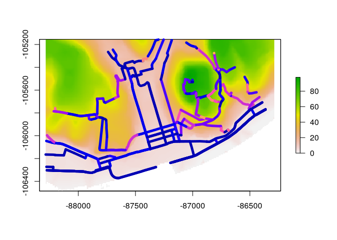
We can now visualise the slopes calculated by the slopes package as
follows:
raster::plot(dem_lisbon_raster)
plot(lisbon_road_segments["slope"], add = TRUE, lwd = 5)
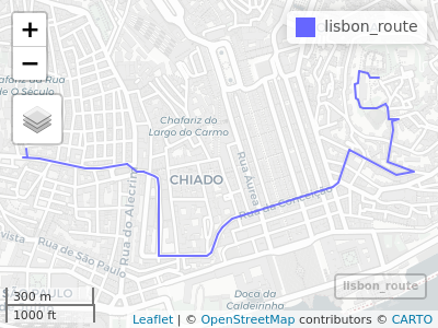
# mapview::mapview(lisbon_road_segments["slope"], map.types = "Esri.WorldStreetMap")Imagine that we want to go from Santa Catarina to the East of the map to the Castelo de Sao Jorge to the West of the map:
mapview::mapview(lisbon_route)We can convert the lisbon_route object into a 3d linestring object as
follows:
lisbon_route_3d = slope_3d(lisbon_route, dem_lisbon_raster)
#> [1] TRUE
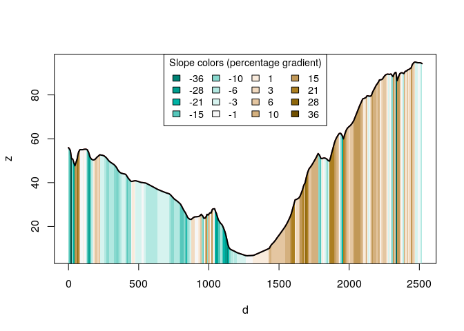
We can now visualise the elevation profile of the route as follows:
plot_slope(lisbon_route_3d)Performance
For this benchmark we will download the following small (< 100 kB)
.tif file:
u = "https://github.com/ITSLeeds/slopes/releases/download/0.0.0/dem_lisbon.tif"
if(!file.exists("dem_lisbon.tif")) download.file(u, "dem_lisbon.tif")
A benchmark can reveal how many route gradients can be calculated per second:
e = dem_lisbon_raster
r = lisbon_road_segments
et = terra::rast("dem_lisbon.tif")
res = bench::mark(check = FALSE,
  slope_raster = slope_raster(r, e, terra = FALSE),
  slope_terra1 = slope_raster(r, e, terra = TRUE),
  slope_terra2 = slope_raster(r, et, terra = TRUE)
)
#> Warning: Some expressions had a GC in every iteration; so filtering is disabled.
res
#> # A tibble: 3 x 6
#>   expression        min   median `itr/sec` mem_alloc `gc/sec`
#>   <bch:expr>   <bch:tm> <bch:tm>     <dbl> <bch:byt>    <dbl>
#> 1 slope_raster   47.6ms   58.1ms      16.5    32.7MB     25.7
#> 2 slope_terra1   55.6ms     61ms      16.5    32.7MB     23.9
#> 3 slope_terra2   44.4ms   53.8ms      11.7    29.4MB     15.6
That is approximately
round(res$`itr/sec` * nrow(r))
#> [1] 4474 4480 3175
routes per second using the raster and terra (the default if
installed, using RasterLayer and native SpatRaster objects) packages
to extract elevation estimates from the raster datasets, respectively.
The message: use the terra package to read-in DEM data for slope
extraction if speed is important.
To go faster, you can chose the simple method to gain some speed at
the expense of accuracy:
e = dem_lisbon_raster
r = lisbon_road_segments
res = bench::mark(check = FALSE,
  bilinear1 = slope_raster(r, e, terra = TRUE),
  bilinear2 = slope_raster(r, et, terra = TRUE),
  simple1 = slope_raster(r, e, method = "simple", terra = TRUE),
  simple2 = slope_raster(r, et, method = "simple", terra = TRUE)
)
#> Warning: Some expressions had a GC in every iteration; so filtering is disabled.
# ?bench::mark
res
#> # A tibble: 4 x 6
#>   expression      min   median `itr/sec` mem_alloc `gc/sec`
#>   <bch:expr> <bch:tm> <bch:tm>     <dbl> <bch:byt>    <dbl>
#> 1 bilinear1    45.8ms   52.9ms      18.9    32.7MB     18.9
#> 2 bilinear2    45.5ms   47.4ms      19.9    29.4MB     19.9
#> 3 simple1      39.4ms   46.9ms      21.7    29.3MB     21.7
#> 4 simple2      38.2ms   51.1ms      20.6    29.4MB     18.8
The equivalent benchmark with the raster package is as follows:
e = dem_lisbon_raster
r = lisbon_road_segments
res = bench::mark(check = FALSE,
  bilinear = slope_raster(r, e, terra = FALSE),
  simple = slope_raster(r, e, method = "simple", terra = FALSE)
)
#> Warning: Some expressions had a GC in every iteration; so filtering is disabled.
# ?bench::mark
res
#> # A tibble: 2 x 6
#>   expression      min   median `itr/sec` mem_alloc `gc/sec`
#>   <bch:expr> <bch:tm> <bch:tm>     <dbl> <bch:byt>    <dbl>
#> 1 bilinear     48.8ms   55.9ms      16.8    32.7MB     20.5
#> 2 simple       43.9ms   49.5ms      13.3    29.3MB     11.4


