Dymos is a framework for the simulation and optimization of dynamical systems within the OpenMDAO Multidisciplinary Analysis and Optimization environment. Dymos leverages implicit and explicit simulation techniques to simulate generic dynamic systems of arbitary complexity.
The software has two primary objectives:
- Provide a generic ODE integration interface that allows for the analysis of dynamical systems.
- Allow the user to solve optimal control problems involving dynamical multidisciplinary systems.
The default installation of the developmental version of Dymos will install the minimum number of prerequisites:
python -m pip install dymos
More advanced installation instructions are available here.
See our overview paper in the Journal of Open Source Software
If you use Dymos in your work, please cite:
@article{Falck2021,
  doi = {10.21105/joss.02809},
  url = {https://doi.org/10.21105/joss.02809},
  year = {2021},
  publisher = {The Open Journal},
  volume = {6},
  number = {59},
  pages = {2809},
  author = {Robert Falck and Justin S. Gray and Kaushik Ponnapalli and Ted Wright},
  title = {dymos: A Python package for optimal control of multidisciplinary systems},
  journal = {Journal of Open Source Software}
}
Online documentation is available at https://openmdao.github.io/dymos/
The first step in simulating or optimizing a dynamical system is to define the ordinary differential equations to be integrated. The user first builds an OpenMDAO model which has outputs that provide the rates of the state variables. This model can be an OpenMDAO model of arbitrary complexity, including nested groups and components, layers of nonlinear solvers, etc.
Dymos solutions are constructed of one or more Phases. When setting up a phase, we add state variables, dynamic controls, and parameters, tell Dymos how the value of each should be connected to the ODE system, and tell Dymos the variable paths in the system that contain the rates of our state variables that are to be integrated.
Dymos's solver-based pseudspectral transcriptions provide the ability to numerically integrate the ODE system it is given. Used in an optimal control context, these provide a shooting method in which each iteration provides a physically viable trajectory.
Dymos currently supports the Radau Pseudospectral Method and high-order Gauss-Lobatto transcriptions. These implicit techniques rely on the optimizer to impose "defect" constraints which enforce the physical accuracy of the resulting trajectories. To verify the physical accuracy of the solutions, Dymos can explicitly integrate them using variable-step methods.
Dymos uses the concept of Phases to support optimal control of dynamical systems. Users connect one or more Phases to construct trajectories. Each Phase can have its own:
- Optimal Control Transcription (Gauss-Lobatto or Radau Pseudospectral)
- Equations of motion
- Boundary and path constraints
Dymos Phases and Trajectories are ultimately just OpenMDAO Groups that can exist in a problem along with numerous other models, allowing for the simultaneous optimization of systems and dynamics.
import numpy as np
import openmdao.api as om
import dymos as dm
import matplotlib.pyplot as plt

# First define a system which computes the equations of motion
class BrachistochroneEOM(om.ExplicitComponent):
    def initialize(self):
        self.options.declare('num_nodes', types=int)

    def setup(self):
        nn = self.options['num_nodes']

        # Inputs
        self.add_input('v', val=np.zeros(nn), units='m/s', desc='velocity')
        self.add_input('theta', val=np.zeros(nn), units='rad', desc='angle of wire')
        self.add_output('xdot', val=np.zeros(nn), units='m/s', desc='x rate of change')
        self.add_output('ydot', val=np.zeros(nn), units='m/s', desc='y rate of change')
        self.add_output('vdot', val=np.zeros(nn), units='m/s**2', desc='v rate of change')

        # Ask OpenMDAO to compute the partial derivatives using complex-step
        # with a partial coloring algorithm for improved performance
        self.declare_partials(of='*', wrt='*', method='cs')
        self.declare_coloring(wrt='*', method='cs', show_summary=True)

    def compute(self, inputs, outputs):
        v, theta = inputs.values()
        outputs['vdot'] = 9.80665 * np.cos(theta)
        outputs['xdot'] = v * np.sin(theta)
        outputs['ydot'] = -v * np.cos(theta)

p = om.Problem()

# Define a Trajectory object
traj = p.model.add_subsystem('traj', dm.Trajectory())

# Define a Dymos Phase object with GaussLobatto Transcription
tx = dm.GaussLobatto(num_segments=10, order=3)
phase = dm.Phase(ode_class=BrachistochroneEOM, transcription=tx)

traj.add_phase(name='phase0', phase=phase)

# Set the time options
phase.set_time_options(fix_initial=True,
                       duration_bounds=(0.5, 10.0))
# Set the state options
phase.add_state('x', rate_source='xdot',
                fix_initial=True, fix_final=True)
phase.add_state('y', rate_source='ydot',
                fix_initial=True, fix_final=True)
phase.add_state('v', rate_source='vdot',
                fix_initial=True, fix_final=False)
# Define theta as a control.
phase.add_control(name='theta', units='rad',
                  lower=0, upper=np.pi)
# Minimize final time.
phase.add_objective('time', loc='final')

# Set the driver.
p.driver = om.ScipyOptimizeDriver()

# Allow OpenMDAO to automatically determine total
# derivative sparsity pattern.
# This works in conjunction with partial derivative
# coloring to give a large speedup
p.driver.declare_coloring()

# Setup the problem
p.setup()

# Now that the OpenMDAO problem is setup, we can guess the
# values of time, states, and controls.
p.set_val('traj.phase0.t_duration', 2.0)

# States and controls here use a linearly interpolated
# initial guess along the trajectory.
p.set_val('traj.phase0.states:x',
          phase.interp('x', ys=[0, 10]),
          units='m')
p.set_val('traj.phase0.states:y',
          phase.interp('y', ys=[10, 5]),
          units='m')
p.set_val('traj.phase0.states:v',
          phase.interp('v', ys=[0, 5]),
          units='m/s')
# constant initial guess for control
p.set_val('traj.phase0.controls:theta', 90, units='deg')

# Run the driver to solve the problem and generate default plots of
# state and control values vs time
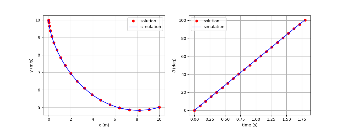
dm.run_problem(p, make_plots=True, simulate=True)

# Load the solution and simulation files.
sol_case = om.CaseReader('dymos_solution.db').get_case('final')
sim_case = om.CaseReader('dymos_simulation.db').get_case('final')

# Plot the results
fig, axes = plt.subplots(nrows=1, ncols=2, figsize=(12, 4.5))

axes[0].plot(sol_case.get_val('traj.phase0.timeseries.states:x'),
             sol_case.get_val('traj.phase0.timeseries.states:y'),
             'ro', label='solution')

axes[0].plot(sim_case.get_val('traj.phase0.timeseries.states:x'),
             sim_case.get_val('traj.phase0.timeseries.states:y'),
             'b-', label='simulation')

axes[0].set_xlabel('x (m)')
axes[0].set_ylabel('y (m/s)')
axes[0].legend()
axes[0].grid()

axes[1].plot(sol_case.get_val('traj.phase0.timeseries.time'),
             sol_case.get_val('traj.phase0.timeseries.controls:theta',
                              units='deg'),
             'ro', label='solution')

axes[1].plot(sim_case.get_val('traj.phase0.timeseries.time'),
             sim_case.get_val('traj.phase0.timeseries.controls:theta',
                              units='deg'),
             'b-', label='simulation')

axes[1].set_xlabel('time (s)')
axes[1].set_ylabel(r'$\theta$ (deg)')
axes[1].legend()
axes[1].grid()

plt.show()