This package is designed for applying formatting on vectors and data frames to make data presentation easier, richer, more flexible and hopefully convey more information.
This document is also translated into 日本語 by @hoxo_m, @dichika and @teramonagi.
The package is available on both GitHub and CRAN.
Install from GitHub:
# install.packages("devtools")
devtools::install_github("renkun-ken/formattable")
Install from CRAN:
install.packages("formattable")Atomic vectors are basic units to store data. Some data can be read more easily with formatting. A numeric vector, for example, stores a group of percentage numbers yet still shows in the form of typical floating numbers. This package provides functions to create data structures with predefined formatting rules so that these objects store the original data but are printed with formatting.
The package provides several typical formattable objects such as percent, comma, currency, accounting and scientific. These objects are essentially numeric vectors with pre-defined formatting rules and parameters. For example,
library(formattable)
p <- percent(c(0.1, 0.02, 0.03, 0.12))
p
## [1] 10.00% 2.00% 3.00% 12.00%
The percent vector is no different from a numeric vector but has a percentage representation as being printed. It works with arithmetic operations and common functions and preserves its formatting.
p + 0.05## [1] 15.00% 7.00% 8.00% 17.00%
max(p)## [1] 12.00%
balance <- accounting(c(1000, 500, 200, -150, 0, 1200))
balance
## [1] 1,000.00 500.00 200.00 (150.00) 0.00 1,200.00
balance + 1000## [1] 2,000.00 1,500.00 1,200.00 850.00 1,000.00 2,200.00
These functions are special cases of what formattable() can do. formattable() applies highly customizable formatting to objects of a wide range of classes like numeric, logical, factor, Date, data.frame, etc. A typical data frame may look more friendly with formattable column vectors. For example,
p <- data.frame(
  id = c(1, 2, 3, 4, 5),
  name = c("A1", "A2", "B1", "B2", "C1"),
  balance = accounting(c(52500, 36150, 25000, 18300, 7600), format = "d"),
  growth = percent(c(0.3, 0.3, 0.1, 0.15, 0.15), format = "d"),
  ready = formattable(c(TRUE, TRUE, FALSE, FALSE, TRUE), "yes", "no"))
p
## id name balance growth ready
## 1 1 A1 52,500 30% yes
## 2 2 A2 36,150 30% yes
## 3 3 B1 25,000 10% no
## 4 4 B2 18,300 15% no
## 5 5 C1 7,600 15% yes
In a typical workflow of dynamic document production, knitr and rmarkdown are powerful tools to render documents with R code to different types of portable documents.
knitr is able to render an RMarkdown document (markdown document with R code chunks) to Markdown document. rmarkdown calls pandoc to render a markdown document to HTML web page. To put a table (data.frame in R) on the page, one may call knitr::kable to produce its markdown representation. By default the resulted table is in a plain theme with no additional formatting. However, in some cases, additional formatting may help clarify the information and make contrast of the data. This package provides functions to produce formatted tables in dynamic documents.
df <- data.frame(
  id = 1:10,
  name = c("Bob", "Ashley", "James", "David", "Jenny",
    "Hans", "Leo", "John", "Emily", "Lee"),
  age = c(28, 27, 30, 28, 29, 29, 27, 27, 31, 30),
  grade = c("C", "A", "A", "C", "B", "B", "B", "A", "C", "C"),
  test1_score = c(8.9, 9.5, 9.6, 8.9, 9.1, 9.3, 9.3, 9.9, 8.5, 8.6),
  test2_score = c(9.1, 9.1, 9.2, 9.1, 8.9, 8.5, 9.2, 9.3, 9.1, 8.8),
  final_score = c(9, 9.3, 9.4, 9, 9, 8.9, 9.25, 9.6, 8.8, 8.7),
  registered = c(TRUE, FALSE, TRUE, FALSE, TRUE, TRUE, TRUE, FALSE, FALSE, FALSE),
  stringsAsFactors = FALSE)
Plain table:
| id | name | age | grade | test1_score | test2_score | final_score | registered |
|---|---|---|---|---|---|---|---|
| 1 | Bob | 28 | C | 8.9 | 9.1 | 9.00 | TRUE |
| 2 | Ashley | 27 | A | 9.5 | 9.1 | 9.30 | FALSE |
| 3 | James | 30 | A | 9.6 | 9.2 | 9.40 | TRUE |
| 4 | David | 28 | C | 8.9 | 9.1 | 9.00 | FALSE |
| 5 | Jenny | 29 | B | 9.1 | 8.9 | 9.00 | TRUE |
| 6 | Hans | 29 | B | 9.3 | 8.5 | 8.90 | TRUE |
| 7 | Leo | 27 | B | 9.3 | 9.2 | 9.25 | TRUE |
| 8 | John | 27 | A | 9.9 | 9.3 | 9.60 | FALSE |
| 9 | Emily | 31 | C | 8.5 | 9.1 | 8.80 | FALSE |
| 10 | Lee | 30 | C | 8.6 | 8.8 | 8.70 | FALSE |
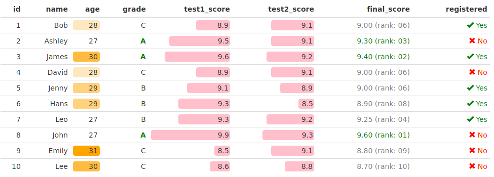
Formatted table with the following visualizations:
- Ages are rendered in gradient.
- All A grades are displayed in green bold.
test1_scoreandtest2_scoreare indicated by horizontal bars and are background-colorized: white (low score) to pink (high score)final_scoreshows score and ranking. Top 3 are green, and others are gray.registeredtexts are transformed to an icon and yes/no text.
library(formattable)

formattable(df, list(
  age = color_tile("white", "orange"),
  grade = formatter("span", style = x ~ ifelse(x == "A",
    style(color = "green", font.weight = "bold"), NA)),
  area(col = c(test1_score, test2_score)) ~ normalize_bar("pink", 0.2),
  final_score = formatter("span",
    style = x ~ style(color = ifelse(rank(-x) <= 3, "green", "gray")),
    x ~ sprintf("%.2f (rank: %02d)", x, rank(-x))),
  registered = formatter("span",
    style = x ~ style(color = ifelse(x, "green", "red")),
    x ~ icontext(ifelse(x, "ok", "remove"), ifelse(x, "Yes", "No")))
))
The icon set used in the table is by GLYPHICONS.com and included in Bootstrap.
formattable will automatically convert to an htmlwidget when in an interactive() context such as the console or RStudio IDE. If you would like to avoid this conversion and see the html table output, please use format_table that calls knitr::kable with formatters or call format with the formattable data.frame object.
This package is under MIT License.
