Interactive Plotting in Scanpy

About

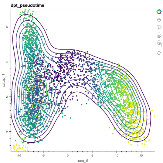
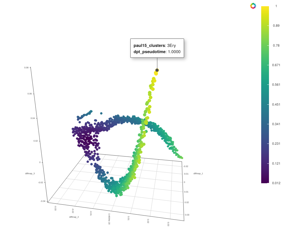
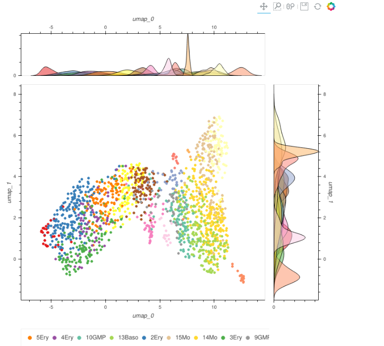
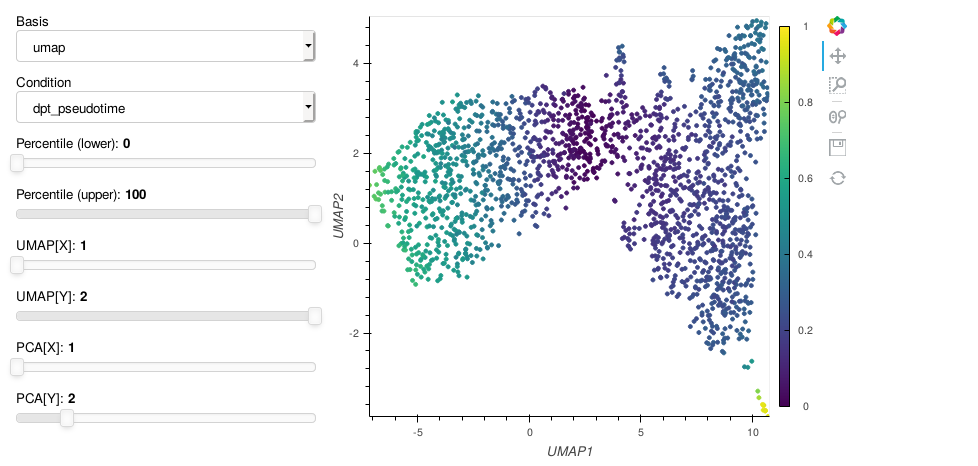
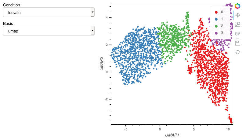
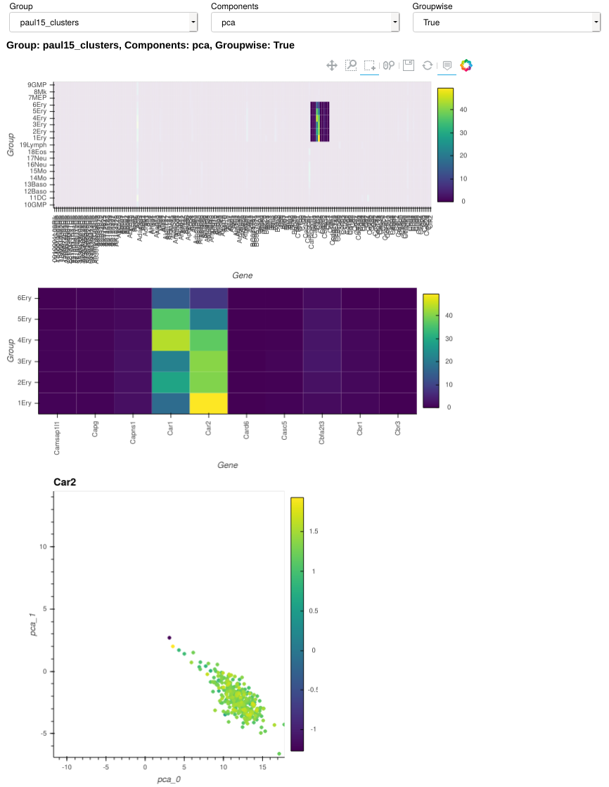
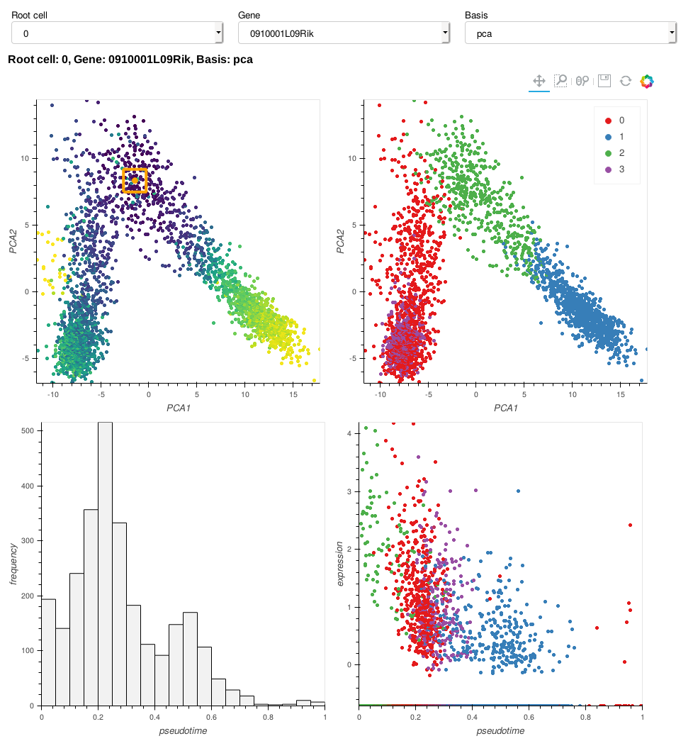
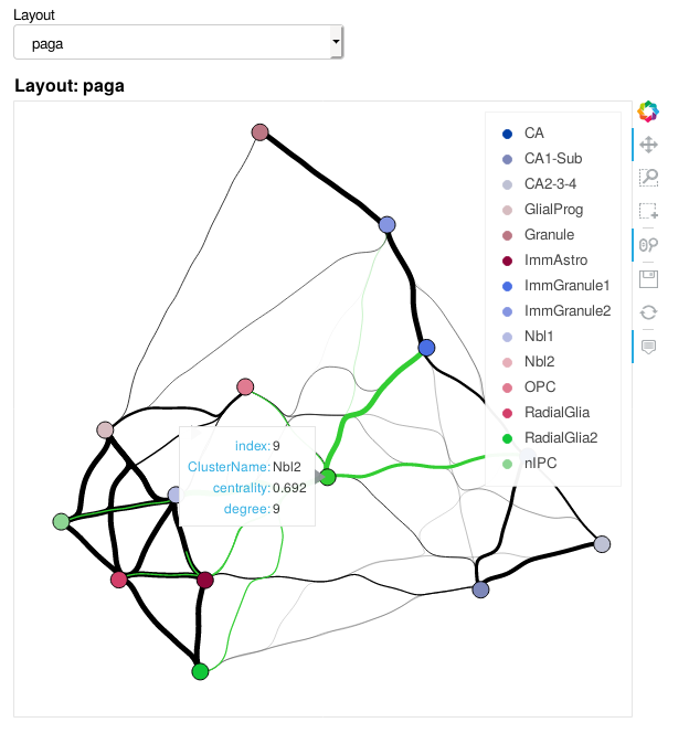
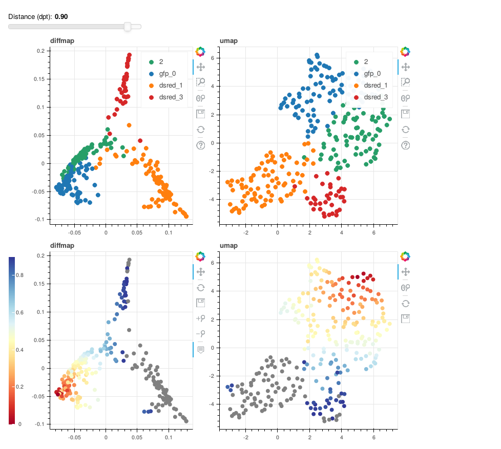
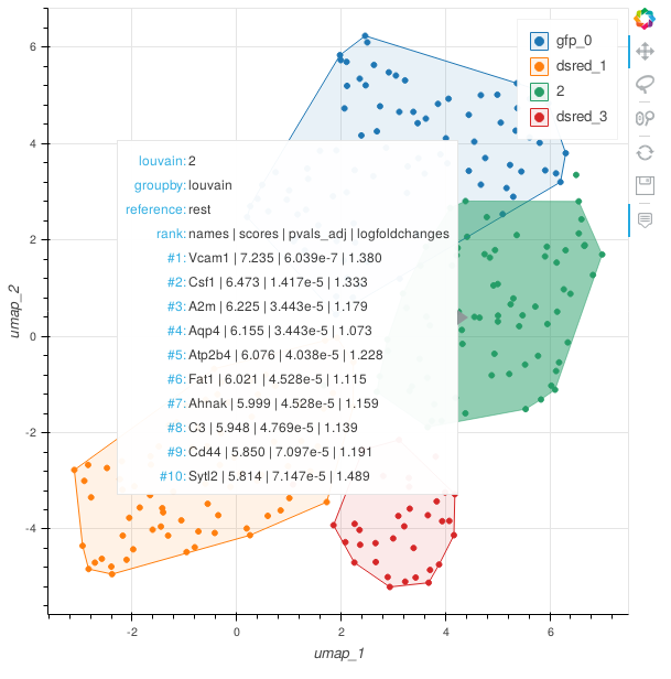
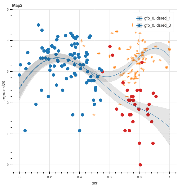
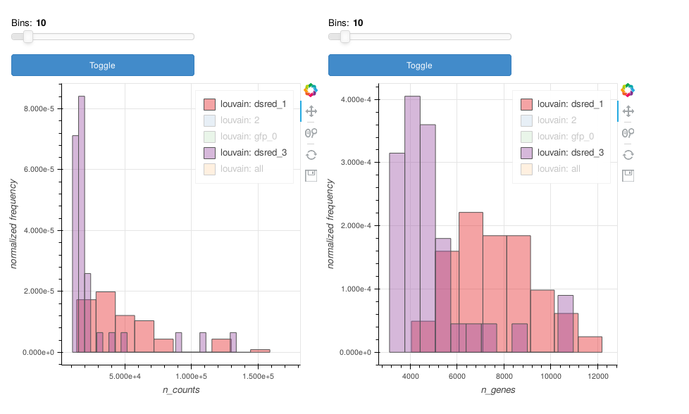
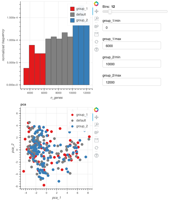
This repository contains 11 different interactive plotting functions, which may be useful during exploratory analysis.

Almost every function provides some information when hovering over the plot and some parts of the plots can be hidden by clicking the legend.

Installation

To install this package, do the following:

conda install nodejs  # >= v6.10.0, for 3D scatterplot
pip install git+https://github.com/theislab/interactive_plotting

For 3D scatterplot, node.js >= v6.10.0 is required. Go to node's website for instructions on how to install it.

Getting Started

We recommend checking out the tutorial notebook. ipl.scatter, ipl.scatterc ipl.dpt can handle large number of cells (100K+).

In your Jupyter Notebook, execute the following lines:

import holoviews as hv  # needed for scatter, scatterc and dpt
hv.extension('bokeh')

import interactive_plotting as ipl  

from bokeh.io import output_notebook
output_notebook()

Gallery

Here are some exemplary figures for each of the plotting functions.

ipl.ex.scatter

ipl.ex.scatter3d

ipl.ex.scatter

ipl.scatter

ipl.scatterc

ipl.ex.heatmap

ipl.dpt

ipl.graph

ipl.link_plot

ipl.highlight_de

ipl.gene_trend

ipl.interactive_hist

ipl.thresholding_hist

Troubleshooting

Notebook size is huge - This has to do with ipl.link_plot and ipl.velocity_plot. Until a fix is found, we suggest removing these figures after you're done using them.
Getting "OPub data rate exceeded" error - Try starting jupyter notebook as following:

jupyter notebook --NotebookApp.iopub_data_rate_limit=1e10

For generating jupyter config file, see here.