Audio signals are all around us. As such, there is an increasing interest in audio classification for various scenarios, from fire alarm detection for hearing impaired people, through engine sound analysis for maintenance purposes, to baby monitoring. Though audio signals are temporal in nature, in many cases it is possible to leverage recent advancements in the field of image classification and use popular high performing convolutional neural networks for audio classification. In this blog post we will demonstrate such an example by using the popular method of converting the audio signal into the frequency domain.
This example is based on a series of blogposts that show how to leverage PyTorch's ecosystem to easily jumpstart your ML/DL project. You can find the Image Classification, Hyperparameter Optimization and the original Audio Classification blogposts here.
The urbansounds dataset consists of the actual data and a csv file containing the metadata. For each sample the csv file keeps track of the location and the label. The data itself is organized into multiple folds, or equal splits of the data. In testing we use 1 fold to validate our model on, all the other folds are used for training.
The first script downloads the data from the official urbansounds sources or in this case a subset that is hosted by ClearML just to play around with. The metadata will be converted into a format that is easier to work with for us and then the files as well as the metadata are uploaded as a ClearML Dataset.
The Dataset is a special sort of task, so we can also generate some interesting logs and plots such as a historgram and attach it to the task just like we would do for any other task.
In order to train a model on the data we want to convert the audio samples (.wav files) to images by creating their mel spectrograms. For more information on how this works read the section below.
In the end we convert each .wav file into a spectrogram image and save the image with the same filename in the same folder. The we create a new ClearML dataset from this dataset. We make it a new version (child) of the previous dataset we made, so the .wav files themselves won't actually be uploaded and just refer to the previously uploaded dataset. ClearML data will only upload the newly created image files.
The metadata from the csv file is again added to the dataset as an artifact. We can just get it as pandas dataframe when we need it.
Finally we get this latest dataset version, download the data itself and get the pandas dataframe containing the metadata. Based on the fold number we divide the data into train and test and train a machine learning model on it. We then log the output scalars and plot a confusion matrix so we can see the model's performance in the ClearML webUI and compare it easily to other experiment runs.
In recent years, Convolutional Neural Networks (CNNs) have proven very effective in image classification tasks, which gave rise to the design of various architectures, such as Inception, ResNet, ResNext, Mobilenet and more. These CNNs achieve state of the art results on image classification tasks and offer a variety of ready to use pre trained backbones. As such, if we will be able to transfer audio classification tasks into the image domain, we will be able to leverage this rich variety of backbones for our needs.
As mentioned before, instead of directly using the sound file as an amplitude vs time signal we wish to convert the audio signal into an image. The following preprocessing was done using this script on the YesNo dataset that is included in torchaudio built-in datasets .
As a first stage of preprocessing we will:
- Read the audio file – using torchaudio
- Resample the audio signal to a fixed sample rate – This will make sure that all signals we will use will have the same sample rate. Theoretically the maximum frequency that can be represented by a sampled signal is a little bit less than half the sample rate (known as the Nyquist frequency). As 20 kHz is the highest frequency generally audible by humans, sampling rate of 44100 Hz is considered the most popular choice. However, in many cases removing the higher frequencies is considered plausible for the sake of reducing the amount of data per audio file. As such, the sampling rate of 20050 Hz has been reasonably popular for low bitrate MP3 files. In our example we will use this sample rate.
- Create a mono audio signal – For simplicity, we will make sure all signals we use will have the same number of channels.
The code for such preprocessing, looks like this:
yesno_data = torchaudio.datasets.YESNO('./data', download=True)
number_of_samples = 3
fixed_sample_rate = 22050
for n in range(number_of_smaples):
    audio, sample_rate, labels = yesno_data[n]
    resample_transform = torchaudio.transforms.Resample(
       orig_freq=sample_rate, new_freq=fixed_sample_rate)
    audio_mono = torch.mean(resample_transform(audio),
       dim=0, keepdim=True)

    plt.figure()
    plt.plot(audio_mono[0,:])
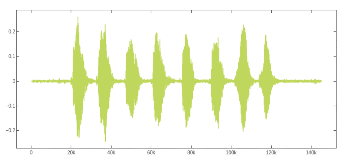
The resulted matplotlib plots looks like this:
Audio signal time series from the YESNO dataset
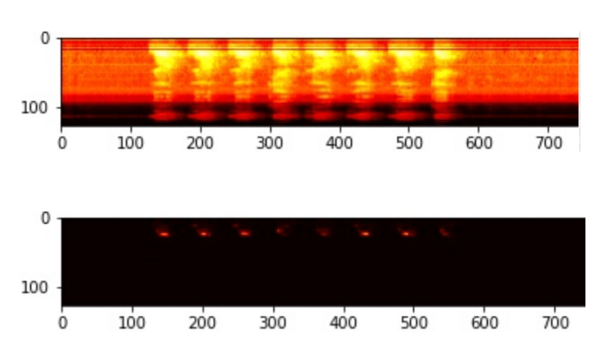
Now it is time to transform this time-series signal into the image domain. We will do that by converting it into a spectogram, which is a visual representation of the spectrum of frequencies of a signal as it varies with time. For that purpose we will use a log-scaled mel-spectrogram. A mel spectrogram is a spectrogram where the frequencies are converted to the mel scale, which takes into account the fact that humans are better at detecting differences in lower frequencies than higher frequencies. The mel scale converts the frequencies so that equal distances in pitch sounded equally distant to a human listener.So let’s use torchaudio transforms and add the following lines to our snippet:
melspectogram_transform =
  torchaudio.transforms.MelSpectrogram(
  sample_rate=fixed_sample_rate, n_mels=128)
melspectogram_db_transform = torchaudio.transforms.AmplitudeToDB()

melspectogram = melspectogram_transform(audio_mono)
plt.figure()
plt.imshow(melspectogram.squeeze().numpy(), cmap='hot')

melspectogram_db=melspectogram_db_transform(melspectogram)
plt.figure()
plt.imshow(melspectogram_db.squeeze().numpy(), cmap='hot')
Now the audio file is represented as a two dimensional spectrogram image:
Mel spectrogram (upper image) and its’ log-scale version (lower image)
That’s exactly what we wanted to achieve. The Audio-classification problem is now transformed into an image classification problem.


