Traffic Sign Recognition

Writeup

Build a Traffic Sign Recognition Project

The goals / steps of this project are the following:

Load the data set (see below for links to the project data set)
Explore, summarize and visualize the data set
Design, train and test a model architecture
Use the model to make predictions on new images
Analyze the softmax probabilities of the new images
Summarize the results with a written report

Rubric Points

Data Set Summary & Exploration

1. Provide a basic summary of the data set. In the code, the analysis should be done using python, numpy and/or pandas methods rather than hardcoding results manually.

I used the numpy to calculate summary statistics of the traffic signs data set:

The size of training set is 34799
The size of the validation set is 4410
The size of test set is 12630
The shape of a traffic sign image is [32, 32, 1]
The number of unique classes/labels in the data set is 43

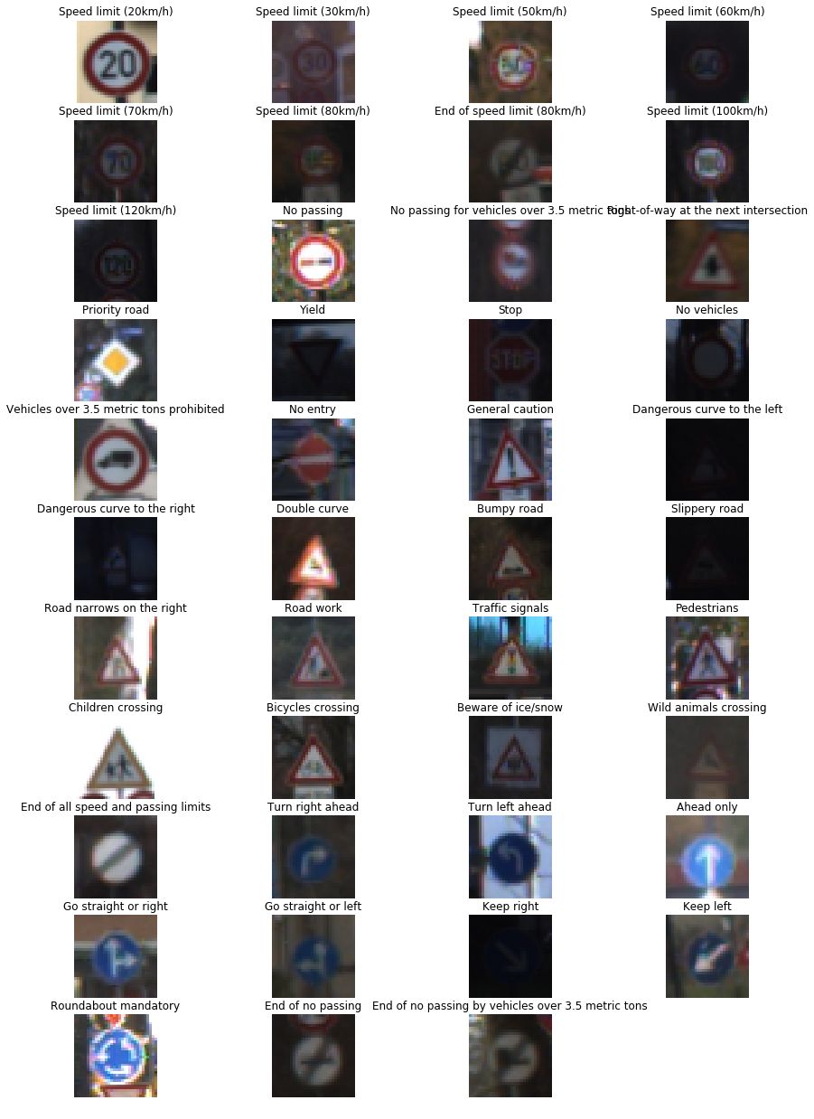
2. Include an exploratory visualization of the dataset.

I created a function "visualize_data()" to visualize the data.

This function plots first image from each category with corresponding label. and it looks like:

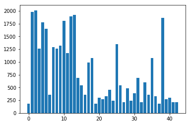
Also, the distribution of count of each label is shown as bar chart

Design and Test a Model Architecture

1. Describe how you preprocessed the image data. What techniques were chosen and why did you choose these techniques? Consider including images showing the output of each preprocessing technique. Pre-processing refers to techniques such as converting to grayscale, normalization, etc. (OPTIONAL: As described in the "Stand Out Suggestions" part of the rubric, if you generated additional data for training, describe why you decided to generate additional data, how you generated the data, and provide example images of the additional data. Then describe the characteristics of the augmented training set like number of images in the set, number of images for each class, etc.)

There are two stages to my preprocessing pipeline:

Convert all the images to grayscale
Standardize all the images to have mean 0 and standard deviation 1

Converting to grayscale is just used to make things simple, though we lose information present in the RGB components.

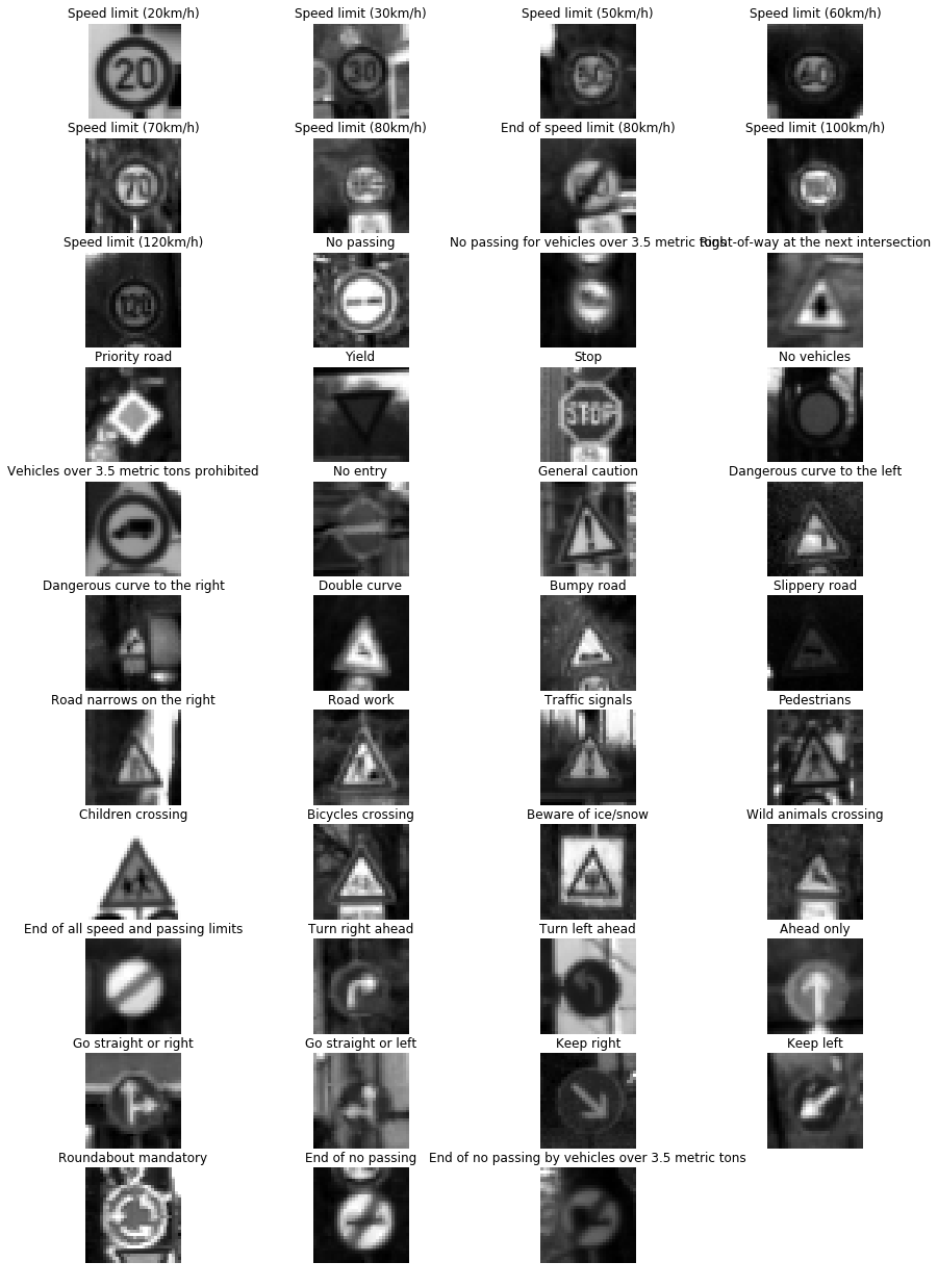
Both of this steps were calculated using a function called pre_process_image(), given a batch of image it calculates gray image for each of the image and then standardizes it by subtracting training dataset mean and training dataset sd.

The output looks something like this, these are the same images as above,

Data Augmentation

Since we have already seen that distribution of input data is not very uniform so it naturally makes sense to augment data and generate more data for class that has small number of images compared to the rest.

Here I have used three transformations 1. Translation, 2. Rotation, 3. Shear This is a very basic implementation using opencv, it takes alot of time to run.

These are implemented as follows:

def translate_img(img):
    """
    Given an input image this function translates it randomly in the range [-3, 7]
    """
    h, w, _ = img.shape
    s1 = (5 * np.random.uniform(-1.0, 1.0)) + 2
    s2 = (5 * np.random.uniform(-1.0, 1.0)) + 2
    #print(s1,s2)
    M = np.array([[1.0, 0.0, s1],
                  [0.0, 1.0, s2]])
    
    dst = cv2.warpAffine(img, M, dsize = (w, h))
    
    return(dst)

def rotate_img(img):
    """
    Given an input image this function rotates it randomly in the range [-30, 30]
    """
    h, w, _ = img.shape
    s = np.random.uniform(-1.0, 1.0) * 30
    if(s == 0):
        s = 30
    M = cv2.getRotationMatrix2D((w/2, h/2), s, 1.2)
    
    dst = cv2.warpAffine(img, M, dsize = (w, h))
    
    return(dst)
    

def shear_img(img):
    """
    Given an input image this function applies shear to it randomly by slightly knocking off basis in the range [-0.2, 0.2]
    """
    h, w, _ = img.shape
    s1 = np.random.uniform(-0.2, 0.2)
    s2 = np.random.uniform(-0.2, 0.2)
    if((s1 == 0.0) & (s2 == 0.0)):
        s1, s2 = 0.2, 0.2
    M = np.array([[1.0, s1, 0.0],
                  [s2, 1.0, 0.0]])
    
    dst = cv2.warpAffine(img, M, dsize = (w, h))
    
    return(dst)

Translated image:

Rotated image

Shear transform

Here I only have generated data for class with less than 720 data points

Why 720?

Because the minimum number of data point were 180 and I have defined 3 transformations, so I didnot want to use one image twice for augmentation. 180 * 3 transformation to each = 720. and this number though small, but is fairly good for the distribution we have here

Distribution of classes after data augmentation

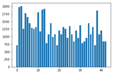
#training samples before data augmentation : 34799 #training samples before data augmentation : 53165

That is 18366 images were created (WOW!)

2. Describe what your final model architecture looks like including model type, layers, layer sizes, connectivity, etc.) Consider including a diagram and/or table describing the final model.

The structure of my model looks like this:

Layer 1:
convolution (6, 5x5x1 filters) (32x32x1 input) (28x28x6 output - valid padding)
ReLU
dropout
max-pool (28x28x6 input) (14x14x6 output)
Layer 2:
convolution (16, 5x5x6 filters) (14x14x6 input) (10x10x16 output)
ReLU
max-pool (10x10x16 input) (5x5x16 output)
Flatten layer (5x5x16 input) (400 output)
dropout
Layer 3:
Fully connected layer (400 input) (120 output)
ReLU
Layer 4:
Fully connected layer (120 input) (84 ouptput)
ReLU
dropout
Layer 5:
Fully connected layer (84 input) (43 output)

3. Describe how you trained your model. The discussion can include the type of optimizer, the batch size, number of epochs and any hyperparameters such as learning rate.

To train the model, I used the code provided at the time of LeNet lab, I used Adam optimizer because it makes training a lot faster and few other improvements over SGD

Batch size = 100
Epochs = 70
Learning rate = 0.0009
dropout probability = 0.5
mu = 0
sigma = 0.1

4. Describe the approach taken for finding a solution and getting the validation set accuracy to be at least 0.93. Include in the discussion the results on the training, validation and test sets and where in the code these were calculated. Your approach may have been an iterative process, in which case, outline the steps you took to get to the final solution and why you chose those steps. Perhaps your solution involved an already well known implementation or architecture. In this case, discuss why you think the architecture is suitable for the current problem.

My final model results were:

validation set accuracy of 94.3 %
test set accuracy of 93.2 %

Most of the time beginners use trial and error method for building NN but if some educated guesses are made then the process of convergence becomes little bit less involved.

As I knew that the training data was adequate enough for this task, I did not use any 1x1 convolution. I used 3 dropout layers to make sure that my model does not overfit, which can be infereed from validation accuracy = 0.943 and test accuracy = 0.932 which are pretty close.

The learning rate and batch size were a bit trail and error, as I increased LR to 0.009 or decreased to 0.00075 the learning did not happen. Accuracy was 0.013 to 0.24. so then I came to middle groung of 0.0009 and it worked.

Though I also want to point out that LR of 0.009 and batch size of 128 gave accuracy of about 90% but it was only with one dropout layer at the 4th layer.

Test a Model on New Images

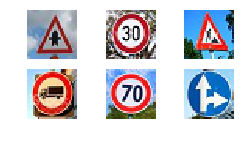
1. Choose five German traffic signs found on the web and provide them in the report. For each image, discuss what quality or qualities might be difficult to classify.

I did not directly get the 32x32 images so these are the downsampled version of original images with varying aspect ratio.

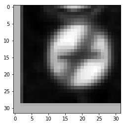
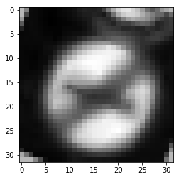
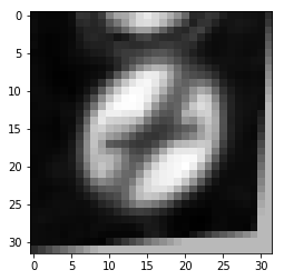
While all images looks clean the last two images are particularly interesting, When I converted these to grayscale, second last image almost looks like a gaussian noise and it is interesting to notice when tested it not only recognized it correctly but the top 5 predictions, not surprisingly were all speed limits

'Speed limit (30km/h)',
'Speed limit (20km/h)',
'Speed limit (50km/h)',
'Speed limit (80km/h)',
'Speed limit (70km/h)'

2. Discuss the model's predictions on these new traffic signs and compare the results to predicting on the test set. At a minimum, discuss what the predictions were, the accuracy on these new predictions, and compare the accuracy to the accuracy on the test set (OPTIONAL: Discuss the results in more detail as described in the "Stand Out Suggestions" part of the rubric).

Here are the results of the prediction:

Image	Prediction
Go straight or right	Go straight or right
Vehicles over 3.5 metric tons prohibited	Vehicles over 3.5 metric tons prohibited
Right-of-way at the next intersection	Right-of-way at the next intersection
Speed limit (70km/h)	Speed limit (70km/h)
Speed limit (30km/h)	Speed limit (30km/h)
Road work	Road work

The model was able to correctly guess 6 of the 6 traffic signs, which gives an accuracy of 100%. comparing this to test set accuracy of 93.2%, I can say that the model is quite robust. if it can give such accuracy on any random image from web then thats a pretty sweet thing.

3. Describe how certain the model is when predicting on each of the five new images by looking at the softmax probabilities for each prediction. Provide the top 5 softmax probabilities for each image along with the sign type of each probability. (OPTIONAL: as described in the "Stand Out Suggestions" part of the rubric, visualizations can also be provided such as bar charts)

The code for making predictions on my final model is:

softmax_logits = tf.nn.softmax(logits)
top_k_pred = tf.nn.top_k(softmax_logits, k = 5)

def predict(images):
    with tf.Session() as sess:
        sess.run(tf.global_variables_initializer())
        saver = tf.train.import_meta_graph('./lenet_drop_0.5_3.meta')
        saver.restore(sess, "./lenet_drop_0.5_3")
        
        softmax_prob = sess.run(softmax_logits, feed_dict={x: images, keep_prob: 1.})
        top_k_prob = sess.run(top_k_pred, feed_dict = {x: images, keep_prob: 1.})
        
        return(top_k_prob)

this gives the top 5 predictions, their index and softmax probabilities.

For all the images given the model was pretty sure of what image contained for example:

Probability	Prediction
.99987	Go straight or right
.00015	Go straight or left
.00	Ahead only
.00	Roundabout mandatory
.00	Dangerous curve to the right

thisisbhavin/German-traffic-sign-classification