- Load, explore, summarize and visualize the German Traffic Sign dataset
- Design, train and test LeNet architecture in TensorFlow
- Use the model to make predictions on new images
- Analyze the softmax probabilities of the new images
- Summarize the results
Link to my project code.
I used the pandas, numpy, and python to calculate summary statistics of the traffic signs data set:
- The size of training set is 34799.
- The size of the validation set is 4410.
- The size of test set is 12630.
- The shape of a traffic sign image is (32, 32, 3).
- The number of unique classes/labels in the data set is 43.
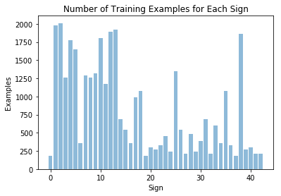
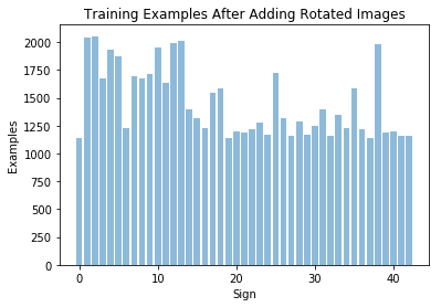
I used a bar chart to visualize the data set:
There is a wide variance in number of examples across the 43 types of signs, ranging from 200 examples to 2000. I also visualized a random image from the training set, to get a feel for what the images looked like:
Data preprocessing was done in several steps. I normalized the image data to 32-bit floating point images:
def norm32(X):
    """
    Normalize image and convert it to 32-bit floating point
    """
    norm = np.float32(128)
    return (X.astype(np.float32) - norm) / norm
This makes sure all the image data has a mean of zero and equal variance, and eliminates the possibility of having data type of image influence the algorithm's learning process. Here is a random image before and after normalization:
I decided to generate additional data because there was such great variance in the number of examples per label (anywhere from 200 to 2000). Labels with a small number of samples would be at high risk of overfitting. To rotate images, I used created the following function:
# To be used in rotation of images
import scipy.ndimage as scnd

def rotate_image(img):
    """
    Rotate image by random angle from Gaussian distribution with a stddev of 7, centered at zero.
    """

    # Create angle from random Gausian distribution with a stddev of 7, centered at zero
    angle = np.random.normal(0., 7.)

    # Rotates pixel array, then essentially houses it inside larger scale blank pixel array
    rotated_img = scnd.interpolation.rotate(img, angle)

    # Rotation creates larger image; crop to 32x32:
    margin = rotated_img.shape[0] - 32 # New rows minus original number of rows
    start_crop = np.floor(margin / 2).astype(int) # Divide by 2 because edge added both sides
    end_crop = start_crop + 32 # Will take 32 rows past bgn_zoomed
    cropped_rotation_img = rotated_img[start_crop:end_crop, start_crop:end_crop, :] # Crop image

    return cropped_rotation_img
This uses scnd.interpolation.rotate(img, angle) to rotate an image array a specificed number of degrees, and then essentially encases that rotated image inside the smallest black rectangle that will fit around it:
The new data was rotated based on an angle chosen randomly from a Gaussian distribution centered at zero, with a standard deviation of 7 degrees. This is to ensure that the majority of the additional images would be extremely similar to their originals, with a few larger rotations mixed in for variance and reducing the possibility of overfitting. This new set of rotated data was then concatenated into the total dataset:
My final model added dropout layers to the LeNet architecture, and slightly adjusted that parameters for processing color images (LeNet is built for grayscale):
| Layer | Description |
|---|---|
| Input | 32x32x3 RGB image |
| Convolution 5x5 | 1x1 stride, valid padding, outputs 28x28x6 |
| RELU | Activation |
| Dropout | Keep Prob = .76 |
| Max pooling | 2x2 stride, outputs 14x14x6 |
| Convolution 5x5 | 1x1 stride, valid padding, outputs 10x10x16 |
| RELU | Activation |
| Dropout | Keep Prob = .76 |
| Max pooling | 2x2 stride, outputs 5x5x16 |
| Flatten | outputs 400 |
| RELU | Activation |
| Dropout | Keep Prob = .76 |
| Fully connected | outputs 120 |
| RELU | Activation |
| Dropout | Keep Prob = .76 |
| Fully connected | outputs 84 |
| RELU | Activation |
| Dropout | Keep Prob = .76 |
| Fully connected | outputs 43 |
| Softmax | outputs classification probabilities |
To train the model, I used the following hyperparameters:
- Learning rate: .000933
- Dropout/Keep Probability: .76
- Epochs: 80
- Batch size: 256
- Optimizer: Adam
My hunch was because LeNet was trained to identify 10 numbers, and we were using it to identify 43 signs, the learning rate would need to be smaller and the number of epochs would need to be larger in order to learn all the nuances. That said, this is my first neural network project, so most of my reasoning for things is "trial and error." For most hyperparameters I just guessed too low, then too high, and repeated that until I reached a happy medium.
I experimented with a learning rate of .00033 for a long time, before returning closer to LeNet's rate of .001 (final rate was .000933). Why the "33" additions? Honestly, because I think Andrew Ng suggested it, but I can neither find where he proposed that nor remember why he said it. But either way it worked.
My intuition for using a 256 batch size was that with a larger number of features, you would need a larger number of examples to better generalize the features. I didn't end up noticing much difference in validation accuracy between a batch size of 128 and 256, but 256 was the only size where I ever could get 100% of my web signs identified. If I was using my personal CPU I'd use a smaller batch size, but working with AWS GPU a batch size of 256 worked well.
I choose the Adam optimizer because it was the most recommended optimizer after a brief web search.
The dropout layers were added in to help keep the network from getting stuck by favoring one specific path. I came to determine a dropout rate of .76 by trial and error.
My final model results were:
- training set accuracy: 1.000
- validation set accuracy: .962
- test set accuracy: .951
I chose the LeNet architecture, which had already been used to identify handwritten numbers. After I adjusted the parameters for color images instead of grayscale, the initial architecture would consistently get stuck at around 89% validation accuracy. My first attempts of improving the accuracy was adding drop out layers. This helped get the accuracy into the low 90's, but the biggest improvements seemed to come from adjusting the learning rate, and preprocessing the dataset.
Because I was training 43 labels instead of just ten like LeNet was set up for, I increased the batch size, number of epochs, and reduced the learning rate. My intuition was that for a human to learn 4 times the labels, you'd have to give it more information, and more time to learn it. I assumed it would be similar for the neural net.
My training accuracy of 1.000, validation accuracy .962, and test accuracy of .951 indicate that the model model's accuracy translates well across different data sets, and is not just specifically fit to the set it was trained on. Plus, it had a 100% accuracy on my new web images.
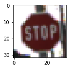
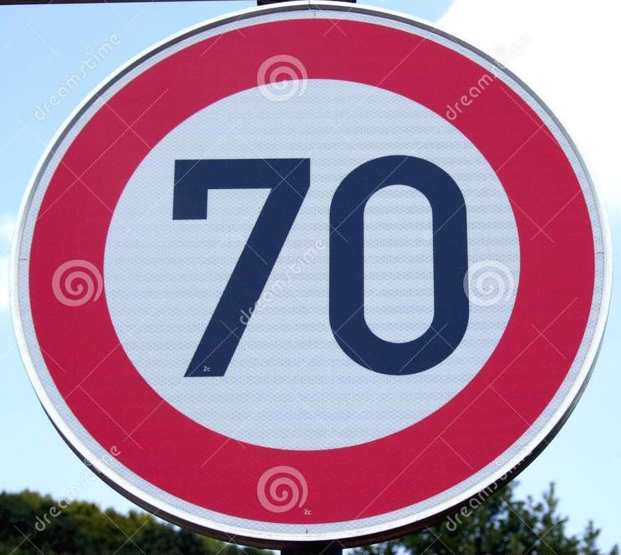
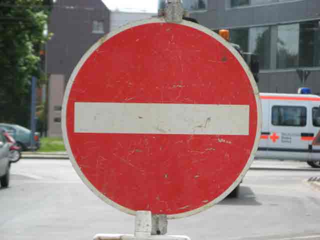
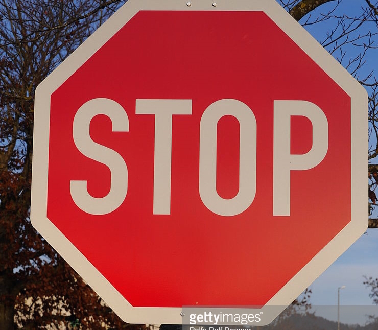
Here are five German traffic signs that I found on the web:
My model was able to classify five of the five signs. To be fair, they were all cropped to look like the dataset images. Images where the sign was rotated significantly or off-center were difficult for the model to handle. Which makes sense, seeing as I did not train the model with those types of images.
In the future, it would probably be helpful to have larger rotations, more obscured signs, signs that weren't centered in the image, add a sliding windows search, or potentially use a more flexible neural network architecture.
Here are the results of the prediction:
| Image | Prediction |
|---|---|
| 30 km/h | 30 km/h |
| 70 km/h | 70 km/h |
| Right Turn Ahead | Right Turn Ahead |
| No Entry | No Entry |
| Stop Sign | Stop Sign |
The model was able to correctly guess five of the five traffic signs, which gives an accuracy of 100%. This compares favorably to the accuracy on the test set of .951.
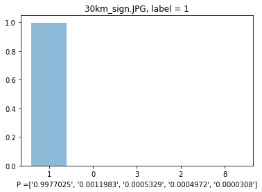
For the first image, the model is certain that this is a 30 km/h sign (probability of 0.99770), and the image does contain a 30 km/h sign. The top five soft max probabilities were:
| Probability | Prediction |
|---|---|
| .99770 | 30 km/h |
| .00120 | 20 km/h |
| .00053 | 60 km/h |
| .00050 | 50 km/h |
| .00003 | 120 km/h |
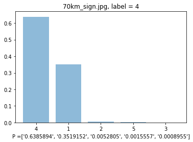
With the second image, the model is relatively sure that this is a 70 km/h sign (probability of 0.63859), and the image does contain a 70 km/h sign. The top five soft max probabilities were:
| Probability | Prediction |
|---|---|
| .63859 | 70 km/h |
| .35192 | 30 km/h |
| .00528 | 50 km/h |
| .00156 | 80 km/h |
| .00090 | 60 km/h |
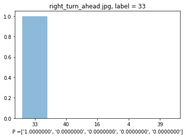
In the third image, the model is absolutely certain that this is a right turn ahead sign (probability of 1.0), and the image does contain a right turn ahead sign. The top five soft max probabilities were:
| Probability | Prediction |
|---|---|
| 1.0 | Right Turn Ahead |
| 0 | Roundabout Mandatory |
| 0 | No vehicles over 3.5 metric tons |
| 0 | 70 km/h |
| 0 | Keep Left |
On the fourth image, the model is absolutely certain that this is a no entry sign (probability of 1.0), and the image does contain a no entry sign. The top five soft max probabilities were:
| Probability | Prediction |
|---|---|
| 1.0 | No Entry |
| 0 | No Passing |
| 0 | Stop Sign |
| 0 | No passing for vehicles over 3.5 tons |
| 0 | Dangerous curve to the right |
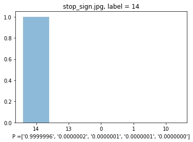
Finally, for the fifth image, the model is certain that this is a stop sign (probability of 0.99999), and the image does contain a stop. The top five soft max probabilities were:
| Probability | Prediction |
|---|---|
| .99999 | Stop Sign |
| .00000 | Yield |
| .00000 | 20 km/h |
| .00000 | 30 km/h |
| .00000 | No passing for vehicles over 3.5 tons |
