Thomas Keggin
This repository aims to serve as a data and code package for getting started with gen3sis (Hagen et al. (2021)). There are other resources available online, so please make sure to have a look around!
-
Gen3sis workshop materials using a dynamic island landscape.
https://github.com/ohagen/gen3sis_yomos_2024 -
Gen3sis wiki page - this includes a tutorial on how to set up a gen3sis project.
https://gitlab.ethz.ch/ele-public/gen3sis_wiki/-/wikis/home
For this tutorial, we will use some modified gen3sis data and code for the marine environment, taken from Keggin et al. (2023). The data and code can both be directly accessed on figshare.
Before reading through this tutorial, please check out Hagen et al. (2021), and familiarise yourself with the structure of the model, the general functions, and their order of operations. It saves me time retyping information here, and saves you time by not getting lost later!
Otherwise, perhaps these figures from the paper will jog your memory:
Overview of the simulation framework:
Overview of a possible study design:
I like to split the workflow into the following steps:
- Wrangle your environmental inputs
- landscape object
- distance matrices
- Configure your simulation
- Run your simulation
- Process your outputs
- Analyse your outputs
Every gen3sis simulation requires two environmental inputs:
-
Landscape object
-
Distance matrices
It’s up to the user to wrangle whatever data they need for their project
into a gen3sis-friendly format. I find it more transparent to do this
manually, using the gdistance package (Etten (2017)) for the distance
matrices. But, it is possible to use the create_input_landscape()
function to convert a list of named rasters into both the landscape
object and distance matrices.
This process can be complex, so here we are using pre-compiled inputs from Keggin et al. (2023), but subset to the Caribbean.
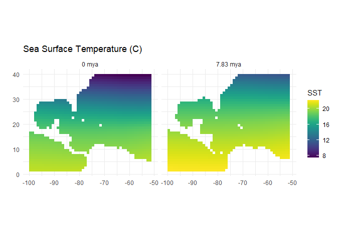
Our landscape object contains sea surface temperature (SST) and depth estimates for every 177 ka from ~ 8 mya until the present (48 time steps) at a 1 degree spatial resolution. The landscapes.rds object itself is a list of two data frames, one for SST and one for depth. Each data frame consists of xy columns for the coordinates, and 48 columns containing the SST and depth values for each time step.
The distance matrices define the geographical distance between every pair of marine cells. This allows us to control how species can disperse across the land(sea)scape. Since the landscape can be different at each time step, we have a distance matrix for each one.
If you’re going to manually set up your landscape object and distance matrices, make sure to follow the file structure and file naming convention - check it out here:
./input/seascapes/.
Let’s have a look at these objects.
landscapes <-
  readRDS("./input/seascapes/landscapes.rds")
List of two data frames,
str(landscapes,
    max.level = 1)
List of 2
$ temp :'data.frame': 1399 obs. of 50 variables:
$ depth:'data.frame': 1399 obs. of 50 variables:
each containing xy coordinates plus SST and depth values for each time step, respectively.
knitr::kable(round(landscapes$temp[1:5,1:10],0),row.names = TRUE)| x | y | 0.00 | 0.17 | 0.33 | 0.50 | 0.67 | 0.83 | 1.00 | 1.17 | |
|---|---|---|---|---|---|---|---|---|---|---|
| 1 | -74 | 40 | 8 | -4 | 8 | -3 | 8 | 1 | 7 | 1 |
| 2 | -72 | 40 | 8 | -3 | 8 | -2 | 8 | 1 | 7 | 2 |
| 3 | -72 | 40 | 8 | -2 | 8 | -1 | 8 | 2 | 7 | 2 |
| 4 | -70 | 40 | 8 | -1 | 8 | 0 | 8 | 2 | 7 | 3 |
| 5 | -70 | 40 | 8 | 0 | 8 | 0 | 8 | 3 | 7 | 3 |
knitr::kable(round(landscapes$depth[1:5,1:10],0),row.names = TRUE)| x | y | 0.00 | 0.17 | 0.33 | 0.50 | 0.67 | 0.83 | 1.00 | 1.17 | |
|---|---|---|---|---|---|---|---|---|---|---|
| 1 | -74 | 40 | -162 | -162 | -156 | -143 | -134 | -117 | -93 | -78 |
| 2 | -72 | 40 | -691 | -691 | -704 | -730 | -734 | -669 | -536 | -451 |
| 3 | -72 | 40 | -1379 | -1379 | -1440 | -1562 | -1605 | -1513 | -1286 | -1195 |
| 4 | -70 | 40 | -2103 | -2103 | -2093 | -2072 | -2013 | -1945 | -1867 | -1854 |
| 5 | -70 | 40 | -2316 | -2316 | -2315 | -2315 | -2269 | -2212 | -2145 | -2114 |
Importantly, row names in these data frames are used to index cells in the simulation - they correspond to row and column names in the distance matrices, and information in the species objects. It is important that these are coherent across your objects - and that you assign them manually/non-automatically.
We can plot these out to see how they correspond to our seascape at different time steps.
Important!
There are some funky quirks to abide by:
Columns must be named.
Columns must be in the order:
$x,y,t_n,t_{n-1},t_{n-2}...t_0$ . I.e., x and y columns, then from the most recent time step into the past.Row names must be assigned non-automatically for both the landscape data frames and distance matrices. This is a characteristic of base R whereby row names assigned automatically can change as you manipulate the object, whereas if you assign them manually they will persist. It is very sneaky and annoying.
These can be either local or full. Local are compressed into a sparse matrix and must be decompressed as the simulation runs, increasing CPU usage. Full are uncompressed, taking up more storage but is less demanding on your CPU resources.
The data here are full. The row and column names correspond to the row names (think of them as cell IDs) in the landscapes data frames. Remember to manually assign the row and column names!
distance_matrix <-
  readRDS("./input/seascapes/distances_full/distances_full_0.rds")

round(distance_matrix[1:10,1:10],0)
1 2 3 4 5 6 7 8 9 10
1 0 86 172 258 344 430 516 602 688 774
2 86 0 86 172 258 344 430 516 602 688
3 172 86 0 86 172 258 344 430 516 602
4 258 172 86 0 86 172 258 344 430 516
5 344 258 172 86 0 86 172 258 344 430
6 430 344 258 172 86 0 86 172 258 344
7 516 430 344 258 172 86 0 86 172 258
8 602 516 430 344 258 172 86 0 86 172
9 688 602 516 430 344 258 172 86 0 86
10 774 688 602 516 430 344 258 172 86 0
Once you have your environment set up, we can think about how you’d like to populate the simulation with species, and determine how these species will behave. This is done through a configuration object. The configuration object is incredibly flexible and can incorporate a lot of complexity depending on your project. This complexity is not necessary though, and we can use a bare-bones configuration to get started.
The configuration object (R object) itself is generated by feeding a
configuration file (an .R script) into the
gen3sis::create_input_config() function - which is called by
gen3sis::run_simulation(). This feels convoluted, but ultimately means
that all we need to do is write an R script containing the required
variable and function definitions.
We have a pre-made configuration file, ./input/configuration_file.R,
that we can read in. But before we do that, let’s make sure we
understand it by going through it’s contents, section by section.
Before setting the simulation functions, we can set up some general variables for the simulation. These are:
-
random_seed: set the seed to control for stochastic functions
-
start_time: specify the starting time step
-
end_time: specify when the simulation should end
-
max_number_of_species: global species limit
-
max_number_of_coexisting_species: local species limit
-
trait_names: specify the traits you would like your species to have!
-
To keep it simple we will include 3 traits describing the relationship between our species and the environment.
-
thermal optimum and standard deviation - more on the thermal response later!
-
depth limit: a hard cut off beyond which our species cannot survive.
-
-
These must correspond to the traits we set up in the initialisation section.
-
-
environmental_ranges: scaling options of environmental values in the landscape object
-
end_of_timestep_observer: a flexible function that allows you to save objects from the simulation environment at the end of each time step. Very useful!
- In this instance we will save species richness per cell, the species object, and the phylogeny at each time step.
# General settings -------------------------------------------------------------
# set the random seed for the simulation
random_seed = 42

# set the starting time step or leave NA to use the earliest/highest timestep
start_time = NA

# set the end time step or leave as NA to use the lates/lowest timestep (0)
end_time = NA

# maximum total number of species in the simulation before it is aborted
max_number_of_species = 1000

# maximum number of species within one cell before the simulation is aborted
max_number_of_coexisting_species = 100

# a list of traits to include with each species
trait_names = c("thermal_optimum",
                "thermal_standard_deviation",
                "depth_limit")

# ranges to scale the input environments with:
# not listed variable:         no scaling takes place
# listed, set to NA:           the environmental variable will be scaled from [min, max] to [0, 1]
# listed with a given range r: the environmental variable will be scaled from [r1, r2] to [0, 1]
environmental_ranges = list()

# a place to inspect the internal state of the simulation and collect additional information if desired
end_of_timestep_observer = function(data, vars, config){
  save_richness()
  save_species()
  save_phylogeny()
}This part took me the longest to figure out. It determines the starting conditions of your simulation and is very flexible!
-
initial_abundance: the starting abundance for both newly colonised cells during the simulation, and those occupied at the beginning of the simulation.
-
create_ancestor_species: this is a function that determines the starting species in the simulation.
-
Inputs: landscape (SST and depth) and a configuration object
-
Output: a species object (list of all extinct and extant species in a simulation).
-
The initial_abundance variable I hope is straightforward, but the
function can be confusing. The gen3sis::create_input_config() function
is reading through the configuration file and slowly building a
configuration object. The gen3sis::create_ancestor_species() function
reads in the landscape object (so we can use it to determine where our
species go) and the partially constructed configuration object
(config). The output is the first species object to be read into the
simulation at time zero.
Remember!
gen3sis::create_ancestor_species()is a custom function, we can set up our species however we like - ultimately, the species object is just a nested list.
We will keep our initialisation as simple as possible without being (I hope) too boring. Let’s start with two imaginary species: one in the Atlantic (Pisces atlanticus), and one the Pacific (Pisces pacificus). To make it interesting, let’s make the Atlantic species a temperature generalist and a depth specialist, and vice versa for the Pacific species.
| species | temperature | depth |
|---|---|---|
| Pisces atlanticus | generalist | specialist |
| Pisces pacificus | specialist | generalist |
Before we get into the function, it might be helpful to have a look at an existing species object - the thing we are trying to create!
species_object <-
  readRDS("./output/configuration_file/species/species_t_47.rds")

str(species_object,
    max.level = 2)
List of 2
$ :List of 5
..$ id : chr "1"
..$ abundance : Named num [1:5] 0.137 0.737 0.997 0.269 0.105
.. ..- attr(*, "names")= chr [1:5] "368" "413" "459" "548" ...
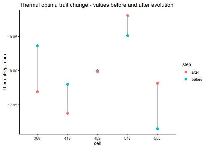
..$ traits : num [1:5, 1:4] 18 18 18 18.1 17.9 ...
.. ..- attr(*, "dimnames")=List of 2
..$ divergence:List of 2
..$ lineage : chr "Pisces_atlanticus"
..- attr(*, "class")= chr "gen3sis_species"
$ :List of 5
..$ id : chr "2"
..$ abundance : Named num [1:42] 0.191 0.167 0.832 0.624 0.699 ...
.. ..- attr(*, "names")= chr [1:42] "1021" "1022" "1069" "1070" ...
..$ traits : num [1:42, 1:4] 21 21 21 21 21 ...
.. ..- attr(*, "dimnames")=List of 2
..$ divergence:List of 2
..$ lineage : chr "Pisces_pacificus"
..- attr(*, "class")= chr "gen3sis_species"
As we can see, the species object is a nested list containing a sub-list for each individual species in the simulation (extinct species will remain in the overall species object, but with null abundance values, etc.). For each species we have the following information:
- id - species ID (new species will be assigned new IDs in serial, automatically)
- abundance - vector of abundances for occupied cells
- traits - matrix of traits for each occupied cell
- divergence - list containing two compression objects for the cell-to-cell divergence values between occupied cells
- lineage - this is a bonus variable I added just in this instance to tag our initial species! This does not usually exist and won’t be used by the simulation.
Whilst we are here, let’s also have a look at one of the trait matrices.
knitr::kable(head(species_object[[1]]$traits))| thermal_optimum | thermal_standard_deviation | depth_limit | dispersal | |
|---|---|---|---|---|
| 368 | 18.03625 | 0.3 | -200 | NA |
| 413 | 17.97982 | 0.3 | -200 | NA |
| 459 | 17.99980 | 0.3 | -200 | NA |
| 548 | 18.05142 | 0.3 | -200 | NA |
| 556 | 17.91502 | 0.3 | -200 | NA |
We can see that there is a column for each trait we specified in the general settings, plus a dispersal trait that gets added by default. Don’t worry about the dispersal trait this time, we won’t be using it!
Manually creating each sub-list for the individual species is tedious.
To make things easier, we can use the gen3sis::create_species()
function to generate each species sub-list instead. Once the individual
species sub-list is created, we can then define the trait values, and
any extras we would like to throw in there.
Hopefully, the following function is now understandable. We start by
pulling out the starting cell IDs for each species, then create each
one. We use gen3sis::create_species() to set up the species sub-list,
then manually set their trait values, plus a bonus lineage name.
# Initialisation ---------------------------------------------------------------
# the initial abundance of a newly colonized cell, both during setup and later when colonizing a cell during the dispersal
initial_abundance = 0.1

# place species within simulation:
create_ancestor_species <- function(landscape, config) {

  #browser()

  seascape <-
    landscape$environment |>
    as_tibble(rownames = "cell")

  coords <-
    landscape$coordinates |>
    as_tibble(rownames = "cell")

  seascape <-
    left_join(seascape,coords,
              by = "cell")

  # define the starting cells for the two species --------
  # species starting in the Atlantic, limited by depth
  Pa_start_cells <-
    seascape |>
    filter(x > -88,x < -84, y > 20, depth > -1000) |>
    pull(cell)

  # species starting in the Pacific, not limited by depth
  Pp_start_cells <-
    seascape |>
    filter(x > -88,x < -84, y < 10) |>
    pull(cell)

  # Remember, the species object is just a list!
  species_object <- list()

  # create the Atlantic species-----------------------------
  species_object[[1]] <-
    gen3sis::create_species(initial_cells = Pa_start_cells,
                            config = config)

  # generate mean thermal niche and standard deviation
  species_object[[1]]$traits[,"thermal_optimum"] <-
    18

  species_object[[1]]$traits[,"thermal_standard_deviation"] <-
    0.3

  # depth trait
  species_object[[1]]$traits[ , "depth_limit"]   <-
    -200

  # tag on a species name
  species_object[[1]]$lineage <-
    "Pisces_atlanticus"

  # create Pacific species ----------------------------------
  species_object[[2]] <-
    gen3sis::create_species(initial_cells = Pp_start_cells,
                            config = config)

  # generate mean thermal niche and standard deviation
  species_object[[2]]$traits[,"thermal_optimum"] <-
    21

  species_object[[2]]$traits[,"thermal_standard_deviation"] <-
    0.1

  # depth trait
  species_object[[2]]$traits[ , "depth_limit"]   <-
    -10000

  # tag on a species name
  species_object[[2]]$lineage <-
    "Pisces_pacificus"

  # output species object
  return(species_object)

}These functions are called every time step, and are the backbone of the simulation. The order below is the order in which they are run.
Speciation in gen3sis is works through a discrete threshold mechanic. The user sets a speciation threshold (in this case, 3) which acts as an upper limit of cell-to-cell differentiation within a species. Once this limit is reached, a new species is formed.
However, how divergence is accrued between isolated cells is highly customisable! For now, every time step at which a pair of cells are isolated, their pairwise differentiation increases by one. For every time step they are connected through a dispersal event, their pairwise differentiation decreases by one.
We assign this by simply returning 1 in the get_divergence_factor()
function.
# Speciation -------------------------------------------------------------------
# threshold for genetic distance after which a speciation event takes place.
# speciation after every timestep : 0.9.
# we are removing the speciation dynamic by setting the threshold to infinity.
divergence_threshold = 3

# factor by which the genetic distance is increased between geographically isolated population of a species
# can also be a matrix between the different population clusters
get_divergence_factor <- function(species, cluster_indices, landscape, config) {

  return(1)
}For every pairwise cell comparison, a dispersal attempt is made. Whether
this attempt is successful or not is determined by comparing the
get_dispersal_values() function output, and the corresponding
geographical distance (distance matrix value) between that pair of
cells. If the cell-to-cell dispersal attempt exceeds the cell-to-cell
value in the corresponding distance matrix for that time step, the
dispersal attempt is a success.
The way in which the dispersal attempt distance value is determined is
highly customisable - and can be determined by environmental variables
and species traits. We will try to keep it simple here by determining
each dispersal attempt through a random pick from a skewed Weibull
distribution, using the stats::rweibull() function.
# Dispersal --------------------------------------------------------------------
# returns n dispersal values
get_dispersal_values <- function(num_draws, species, landscape, config) {

  return(
    rweibull(num_draws,
             shape = 2,
             scale = 500)
  )
}
Which we can visualise:
Every time step we can change the trait values of each species, which is again highly flexible! We will keep this simple by changing the thermal optima of each species randomly through drawing values from a normal distribution.
Let’s call this random, undirected phenotypic mutation - the trait does not track the environment. But you could set it up so that it does!
# Evolution --------------------------------------------------------------------
# mutate the traits of a species and return the new traits matrix
apply_evolution <- function(species, cluster_indices, landscape, config){

  #browser()

  traits <-
    species[["traits"]]

  traits[,"thermal_optimum"] <-
    traits[,"thermal_optimum"] + rnorm(length(traits[,"thermal_optimum"]),
                                       mean=0,
                                       sd=0.04)

  return(traits)
}The most complex looking, but most intuitive function we will use! We load in the existing abundance values for each cell in a species, modify them, then return a new set of abundance values.
In this implementation, each cell has a minimum abundance of 0, and a maximum abundance of 1.
A cell with an abundance of 0 at the end of this function will go locally extinct!
In our case we have three traits that determine the local abundance of a species:
-
Thermal optimum
-
Thermal standard deviation
-
Depth limit
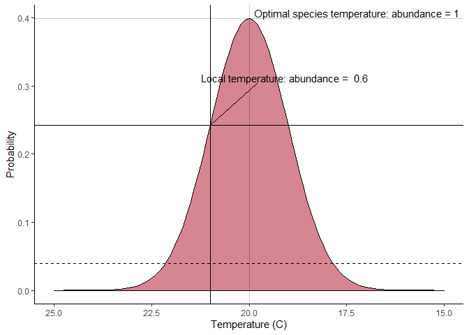
We use the thermal optimum (mean) and standard deviation to describe a normal distribution to act as an abundance thermal response to temperature. As the distribution probability decays away from the mean (thermal optimum), so does the abundance in that cell. If the resulting abundance is below 0.1, we drive that cell to extinction.
Let’s look at an example where the environmental temperature is 21 C, the thermal optimum is 20 C, and the standard deviation is 1 C. The horizontal dashed line is the 0.1 extinction threshold.
More simply, the depth limit acts as a hard cut off for abundance. If the depth of the cell is shallower than the depth limit, nothing happens. If it is deeper, that cell is driven to extinction (abundance = 0).
# Ecology ----------------------------------------------------------------------
# called for every cell with all occuring species, this function calculates who survives in the current cells
# returns a vector of abundances
# set the abundance to 0 for every species supposed to die
apply_ecology <- function(abundance, traits, local_environment, config) {

  #browser()

  new_abundance <-

    # trait information
    dplyr::as_tibble(traits) |>

    # environmental information
    cbind(dplyr::as_tibble(local_environment)) |>

    # ecology calculations
    dplyr::mutate(

      # start abundance
      start_abundance = abundance,

      # the distribution density if the species' niche perfectly fits the temperature
      optimal_density = dnorm(thermal_optimum,
                              mean = thermal_optimum,
                              sd = thermal_standard_deviation),

      # the distribution density given the distance between species niche and temperature
      species_density = dnorm(thermal_optimum,
                              mean = temp,
                              sd = thermal_standard_deviation),

      # determine the abundance
      end_abundance = species_density/optimal_density,

      # drive to (local) extinction if abundance is below 10%
      end_abundance = ifelse(end_abundance < 0.1,
                             0,
                             end_abundance),

      # drive to (local) extinction if the temperature is completely unsuitable
      end_abundance = ifelse(species_density == 0,
                             0,
                             end_abundance),

      # drive to (local) extinction if the depth is unsuitable
      end_abundance = ifelse(depth < depth_limit,
                             0,
                             end_abundance)
    ) |>

    # extract end abundance only
    dplyr::pull(end_abundance)

  # assign cell names
  names(new_abundance) <- names(abundance)

  # fin
  return(new_abundance)
}
And that’s it! Please have a look at the configuration file itself to
see the full layout: ./inputs/configuration_file.R.
If you have hawk-like code-reading eyes, you might have noticed the
browser()function hashed out at the start of each function. Debugging the config can be a nightmare, thebrowser()function will help!
We finally have our configuration file, landscapes, and distance
matrices, and are ready to run our simulation. This is done using the
gen3sis::run_smulation() function, which we can run in the console.
Our current implementation shouldn’t be too heavy - give it a go
yourself!
run_simulation(
  config = "./input/configuration_file.R",
  landscape = "./input/seascapes/",
  output_directory = "./output/",
  call_observer = "all",
  enable_gc = TRUE,
  verbose = 1
)
And that’s the bulk of it. Once you have your outputs, it’s really up to the user to decide what they’d like to do with them. For fun, I’ve continued a bit below by having a quick look at the outputs we get from our practice simulation.
This is just the beginning - most users run batches of gen3sis simulations. This can be done by building a configuration file template and generating many parameter variants of that template. It is outside the scope of what we’re doing here though.
The bulk of the information from the simulation is contained in the species objects. We saved the species objects from each time step. Below is a block of code that extracts this species information and compiles it all into a single data frame for analysis. It includes a couple of custom Thomas Keggin functions - feel free to steal them.
# functions
dir_fun <-
  "./scripts/functions/"

for(f in list.files(dir_fun)){

  source(paste0(dir_fun,f))
}

# vector of species objects (one for each time step)
species_files <-
  list.files("./output/configuration_file/species/")

# container for species data frames for each time step
species_dfs <-
  vector("list",length(species_files))

# loop through species objects
for(file in 1:length(species_files)){

  # load in and apply species data frame function (converts species object into
  # a data frame, excluding the divergence information)
  species_dfs[[file]] <-
    speciesDF(
      species_object = readRDS(paste0("./output/configuration_file/species/",
                                      species_files[file])))

  # skip where all species are extinct :(
  if(dim(species_dfs[[file]])[1] > 0){

    species_dfs[[file]] <-
      species_dfs[[file]] |>
      mutate(timestep = parse_number(species_files[file]),
             .before = 1)
  }
}

# combine data frames
metrics_cell <-
  do.call(rbind.data.frame,species_dfs) |>
  as_tibble()

# export -----------------------------------------------------------------------
write_csv(metrics_cell,
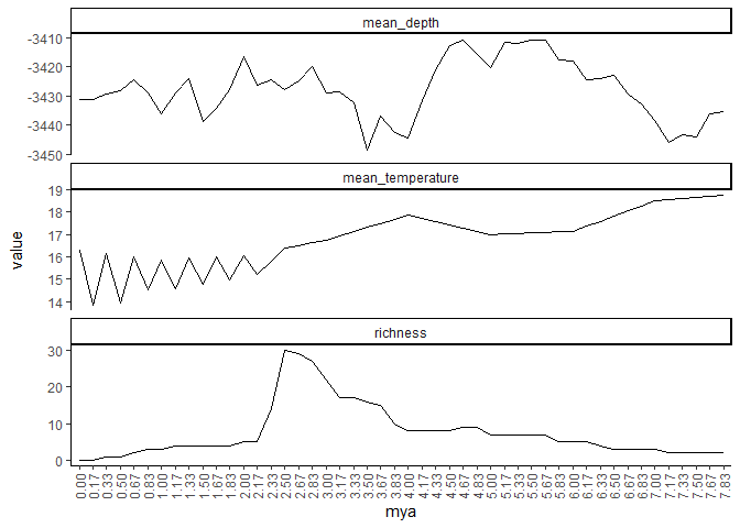
"./results/species_output.csv") #outputWe can see how species richness builds until the onset of the interglacial periods, which eventually drive both of our lineages to extinction.
temperature <-
  landscapes$temp |>
  as_tibble(rownames = "cell") |>
  pivot_longer(cols = c(!cell:y),
               names_to = "mya",
               values_to = "temperature") |>
  group_by(mya) |>
  reframe(mean_temperature = mean(temperature,na.rm=T))

depth <-
  landscapes$depth |>
  as_tibble(rownames = "cell") |>
  pivot_longer(cols = c(!cell:y),
               names_to = "mya",
               values_to = "depth") |>
  group_by(mya) |>
  reframe(mean_depth = mean(depth,na.rm=T))

years_to_timesteps <-
  data.frame(mya = colnames(landscapes$depth[,-c(1:2)]),
             timestep = 0:47)

richness_v_t <-
  metrics_cell |>
  left_join(years_to_timesteps,by="timestep") |>
  group_by(mya) |>
  reframe(richness = length(unique(species)))

global_extinction <-
  data.frame(mya = years_to_timesteps$mya[!years_to_timesteps$mya %in% richness_v_t$mya],
             richness = 0)

richness_v_t <-
  rbind(richness_v_t,
        global_extinction)

plot_me <-
  richness_v_t |>
  left_join(temperature,by = "mya") |>
  left_join(depth,by = "mya") |>
  pivot_longer(cols = c(!mya))


ggplot(plot_me) +
  geom_line(aes(x = mya,
                 y = value,
                group=1))+
  facet_wrap(~name,ncol = 1,scales = "free_y") +
  theme_classic() +
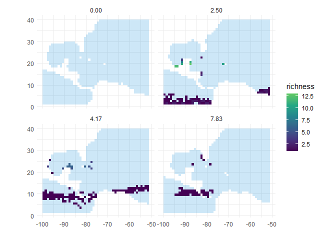
theme(axis.text.x = element_text(angle = 90, vjust = 0.5, hjust=1))We can also manipulate the landscapes and cell metrics to plot out spatial patterns - let’s have a look at species richness pattern at particular points in our simulation’s history.
It looks like Pisces pacificus manages to colonise the Atlantic through its high depth tolerance, but can’t ride out the harsh temperature fluctuations of the interglacials.
Conversely, Pisces atlanticus does a better job at surviving the thermal stress, but with a more fragmented distribution due to its depth limitations, causing it to speciate more frequently. Sadly, this lineage also goes extinct.
Play with the trait values in the configuration
gen3sis::create_ancestor_species() function to see how their fates
could be different.
target_step <-
  c(0,15,25,47)

ocean <-
  landscapes$depth |>
  as_tibble(rownames = "cell") |>
  pivot_longer(cols = !c(x,y,cell),
               names_to = "mya",
               values_to = "depth") |>
  left_join(years_to_timesteps,by = "mya")

# start richness
richness <-
  metrics_cell |>
  group_by(timestep,cell) |>
  reframe(richness = length(unique(species)))

plot_me <-
  left_join(ocean,richness,by = join_by(cell, timestep)) |>
  filter(timestep %in% target_step,
         !is.na(depth))

ggplot(plot_me) +

  geom_tile(aes(x=x,y=y),fill = "#0487D9",alpha = .2) +
  geom_tile(aes(x=x,y=y,fill = richness)) +
  facet_wrap(~mya) +
  scale_fill_viridis_c(na.value = "transparent",end = 0.75) +
  coord_fixed() +
  theme_minimal() +
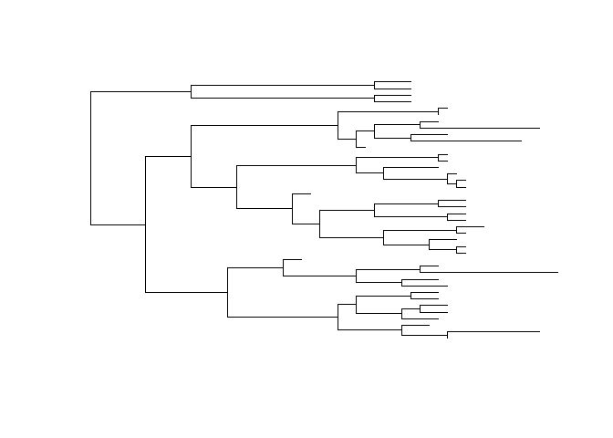
xlab("")+ylab("")We can also pull the phylogeny from the entire simulation, if we’d like to dig into the world of in-silico phylogeography!
phylogeny <-
  read.nexus(paste0("./output/configuration_file/phy.nex"))

phylogeny$edge.length <-
  phylogeny$edge.length+1

plot.phylo(phylogeny,
show.tip.label = FALSE)Etten, Jacob van. 2017. “R Package Gdistance: Distances and Routes on Geographical Grids.” Journal of Statistical Software 76 (13): 1–21. https://doi.org/10.18637/jss.v076.i13.
Hagen, O., B. Fluck, F. Fopp, J. S. Cabral, F. Hartig, M. Pontarp, T. F. Rangel, and L. Pellissier. 2021. “Gen3sis: A General Engine for Eco-Evolutionary Simulations of the Processes That Shape Earth’s Biodiversity.” PLOS Biology 19 (7): 31. https://doi.org/10.1371/journal.pbio.3001340.
Keggin, Thomas, Conor Waldock, Alexander Skeels, Oskar Hagen, Camille Albouy, Stéphanie Manel, and Loïc Pellissier. 2023. “Diversity Across Organisational Scale Emerges Through Dispersal Ability and Speciation Dynamics in Tropical Fish.” BMC Biology 21 (1): 282. https://doi.org/10.1186/s12915-023-01771-3.
