beer

The aim of beer is to make it easier to automatically train and analyse data.

Usage

The main method is train.models, used to train multiple models automatically and visualise on demand.

There are two options to train multiple models automatically: either by providing more than one distribution family (only applicable for classifiers which take a distribution family) or by replacing a part of the formula. The former is passed to train.models with the parameter fam, the latter with parameter replacement. The first example shows the latter, the second the former.

First example:

t.m = train.models("Sepal.Length ~ Sepal.Width + %",
					iris, 
					algo="lm.linear_model",
					replacement=c("Petal.Length","Petal.Width","Species"))

It trains a linear regression by using lm on the iris dataset. The algorithm is set by passing lm.linear_model in parameter algo. Currently supported are

lm.linear_model (lm)
glm.linear_model (glm)
lmer.linear_model (lmer from package lme4)
nlme.linear_model (nlme from package lme4).

Those are easily extendable, which is discussed under Section Extensability.

The first parameter is the formula, nothing changes except for the special character %. It is used as a replacement character. Parameter replacement takes a vector of column names of the passed data (in the first example iris) that should replace % in the formula. As for now, only one replacement per formula is possible. If no % is used in the formula, no replacement can be used. The parameter becomes optional.

In the first example three lm-models are trained with the formulas and returned

Sepal.Length ~ Sepal.Width + Petal.Length
Sepal.Length ~ Sepal.Width + Petal.Width
Sepal.Length ~ Sepal.Width + Species

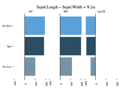
Since lm does not take a distribution, only three models in total are trained. By default the results of the three models are visualised, printed as a table and an anova is run on it. The result of the visualisation can be seen here:

The second example uses glm to train the previous formula but also providing three distribution families.

t.m = train.models("Sepal.Length ~ Sepal.Width + %", 
					iris, 
					algo="glm.linear_model",
					fam=c("gaussian","inverse.gaussian","Gamma"), 
					replacement=c("Petal.Length","Petal.Width","Species"))

Now what happens is it runs all possible combinations of the family and formula. Three replacements for the formula and three families equals nine trained models.

Sepal.Length ~ Sepal.Width + Petal.Length with gaussian
Sepal.Length ~ Sepal.Width + Petal.Length with inverse.gaussian
Sepal.Length ~ Sepal.Width + Petal.Length with Gamma
Sepal.Length ~ Sepal.Width + Petal.Width with gaussian
Sepal.Length ~ Sepal.Width + Petal.Width with inverse.gaussian
Sepal.Length ~ Sepal.Width + Petal.Width with Gamma
Sepal.Length ~ Sepal.Width + Species with gaussian
Sepal.Length ~ Sepal.Width + Species with inverse.gaussian
Sepal.Length ~ Sepal.Width + Species with Gamma

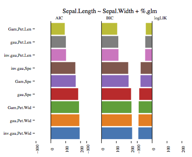
The visualisation again shows AIC, BIC and logLIK values for all nine models:

As mentioned before, the output also includes a table of the performances of each model (AIC, BIC, logLIK) as well as the anova analysis. Both table outputs are shown below.

Performance Table
[1] "Sepal.Length ~ Sepal.Width + %"
                AIC      BIC      logLIK   
Gam,Pet.Len     93.58843 105.631  -42.79422
gau,Pet.Len     101.0255 113.068  -46.51275
inv.gau,Pet.Len 102.3047 114.3473 -47.15237
inv.gau,Spe     164.8211 179.8743 -77.41055
Gam,Spe         167.318  182.3712 -78.65899
gau,Spe         183.9366 198.9898 -86.96829
Gam,Pet.Wid     189.5796 201.6221 -90.78979
gau,Pet.Wid     191.8207 203.8633 -91.91036
inv.gau,Pet.Wid 194.147  206.1896 -93.07352


ANOVA
Analysis of Deviance Table

Model 1: Sepal.Length ~ Sepal.Width + Petal.Length
Model 2: Sepal.Length ~ Sepal.Width + Petal.Length
Model 3: Sepal.Length ~ Sepal.Width + Petal.Length
Model 4: Sepal.Length ~ Sepal.Width + Petal.Width
Model 5: Sepal.Length ~ Sepal.Width + Petal.Width
Model 6: Sepal.Length ~ Sepal.Width + Petal.Width
Model 7: Sepal.Length ~ Sepal.Width + Species
Model 8: Sepal.Length ~ Sepal.Width + Species
Model 9: Sepal.Length ~ Sepal.Width + Species
  Resid. Df Resid. Dev Df Deviance
1       147    16.3288            
2       147     0.4640  0  15.8648
3       147     0.0850  0   0.3789
4       147    29.9111  0 -29.8261
5       147     0.8794  0  29.0317
6       147     0.1569  0   0.7226
7       146    28.0037  1 -27.8468
8       146     0.7482  0  27.2555
9       146     0.1273  0   0.6209

Once the model is stored in a variable (in the examples it is stored t.m), the generic methods plot, print and anova can be used. E.g. plot(t.m) results in a ggplot2 plot of AIC, BIC and logLik, showed in the two example images.

For more examples and the anova / table output check example(train.models).

Extensability

Adding another classifier is simple. Create a function which name ends in ".linear_model". E.g. "gglm.linear_model". This is passed in train.models as parameter algo.

The function should follow the four .linear_model-functions in models.r and should use function linear_model to train the model. For now the latter is only a precaution in case linear_model will be used for more than just training in the future.

Example time:

gbm.linear_model = function(formula,data,fam,...){
	linear_model(formula,data,gbm,distribution=fam,...)    
}

t.m = train.models("Sepal.Length ~ Sepal.Width + %", 
                   iris, 
                   algo="gbm.linear_model",
                   fam=c("gaussian","multinomial"), 
                   replacement=c("Petal.Length","Petal.Width","Species"),output=F)

thomaskern/beer

beer

Usage

Extensability