thorinf/bayesian-flow-pytorch

Implementation of Bayesian Flow, from the Bayesian Flow Networks paper, in Pytorch

Bayesian Flow - Pytorch

A standalone library for adding Bayesian Flow in Pytorch.

Install

$ pip install -e .

Features

Continuous Data

• Discrete Time Loss
• Continuous Time Loss
• Sampler
• Example
• Self-Conditioning

Discretised Data

• Discrete Time Loss
• Continuous Time Loss
• Sampler
• Example
• Self-Conditioning

Discrete Data

• Discrete Time Loss
• Continuous Time Loss
• Sampler
• Example
• Self-Conditioning

Utilised By

bayesian-flow-mnist: A simple Bayesian Flow model for MNIST in Pytorch. Replicated the binarised MNIST generation, and can also generate MNIST as continuous data.

Usage

import torch
from bayesian_flow_torch import BayesianFlow

# Instantiate your torch model
model = ...

# Instantiate Bayesian Flow for continuous data
# Sigma must be set
bayesian_flow = BayesianFlow(sigma=0.001)

# Compute the continuous data continuous time loss
loss = bayesian_flow.continuous_data_continuous_loss(model=..., target=..., model_kwargs=...)

# Generate samples from the model 
samples = bayesian_flow.continuous_data_sample(model=..., size=..., num_steps=..., device=..., model_kwargs=...)

import torch
from bayesian_flow_torch import BayesianFlow

# Instantiate your torch model
model = ...

# Instantiate Bayesian Flow for discrete data
# Number of classes and Beta must be set
# NOTE: There appears to be an inverse relationship between number of classes and Beta
# For binary data, i.e. `num_classes=2`, you may also set `reduced_features_binary=True` to reduce the features to 1
bayesian_flow = BayesianFlow(num_classes=..., beta=..., reduced_features_binary=...)

# Compute the discrete data continuous time loss for the batch
# Target may contain class indices, or class probabilities [0, 1]. 
# Target probalities final dimension must match number of classes, unless `reduced_features_binary=True` where it's 1.
loss = bayesian_flow.discrete_data_continuous_loss(model=..., target=..., model_kwargs=...)

# Generate samples from the model 
# Size should not include the number of classes
samples = bayesian_flow.discrete_data_sample(model=..., size=..., num_steps=..., device=..., model_kwargs=...)

As noted above, there appears to be an inverse relationship between num_classes and beta. Within the discrete loss, theta represents the softmax of a noised simplex, and is the input to the model. If beta is too large with respect to the num_classes, theta will effectively match the ground truth distribution for many of the time-steps. If the theta distribution consistently matches the ground truth, there is nothing to learn. By looking at values of theta you may be able to identify if the beta is low enough to adequately noise the simplex such that there is a loss of information between the ground truth and theta.

Examples

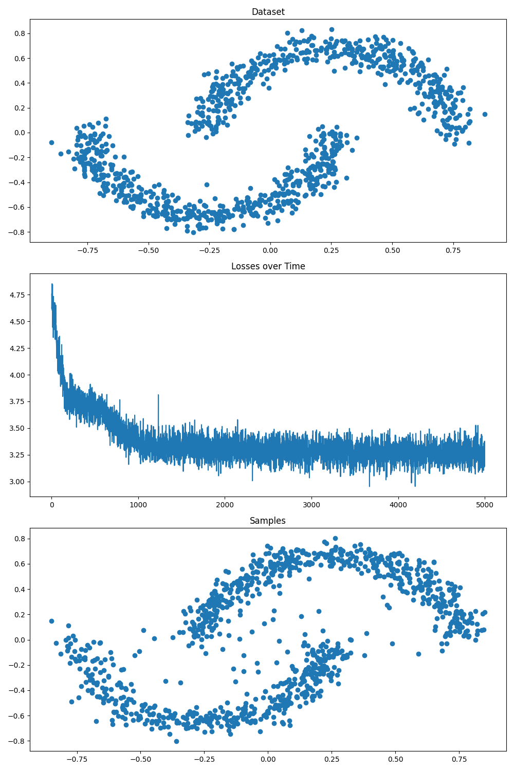
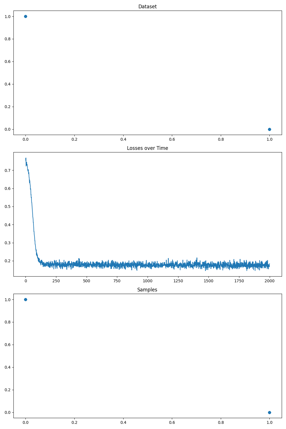
In the examples directory are simple toy examples.

Figure 1. Continuous Data: 'Two Moons' Coordinates

Figure 2. Discrete Data: Predict XOR Logic

Citations

@misc{graves2023bayesian,
      title={Bayesian Flow Networks}, 
      author={Alex Graves and Rupesh Kumar Srivastava and Timothy Atkinson and Faustino Gomez},
      year={2023},
      eprint={2308.07037},
      archivePrefix={arXiv},
      primaryClass={cs.LG}
}