Interpolations

NEWS This package is currently under new maintainership. Please be patient while the new maintainer learns the new package. If you would like to volunteer, please mention this in an issue.

NEWS v0.9 was a breaking release. See the news for details on how to update.

This package implements a variety of interpolation schemes for the Julia language. It has the goals of ease-of-use, broad algorithmic support, and exceptional performance.

Currently this package's support is best for B-splines and also supports irregular grids. However, the API has been designed with intent to support more options. Initial support for Lanczos interpolation was recently added. Pull-requests are more than welcome! It should be noted that the API may continue to evolve over time.

Other interpolation packages for Julia include:

Some of these packages support methods that Interpolations does not, so if you can't find what you need here, check one of them or submit a pull request here.

At the bottom of this page, you can find a "performance shootout" among these methods (as well as SciPy's RegularGridInterpolator).

Installation

Just

using Pkg
Pkg.add("Interpolations")

from the Julia REPL.

Example Usage

Create a grid xs and an array A of values to be interpolated

xs = 1:0.2:5
f(x) = log(x)
A = [f(x) for x in xs]

Create linear interpolation object without extrapolation

interp_linear = LinearInterpolation(xs, A)
interp_linear(3) # exactly log(3)
interp_linear(3.1) # approximately log(3.1)
interp_linear(0.9) # outside grid: error

Create linear interpolation object with extrapolation

interp_linear_extrap = LinearInterpolation(xs, A,extrapolation_bc=Line()) 
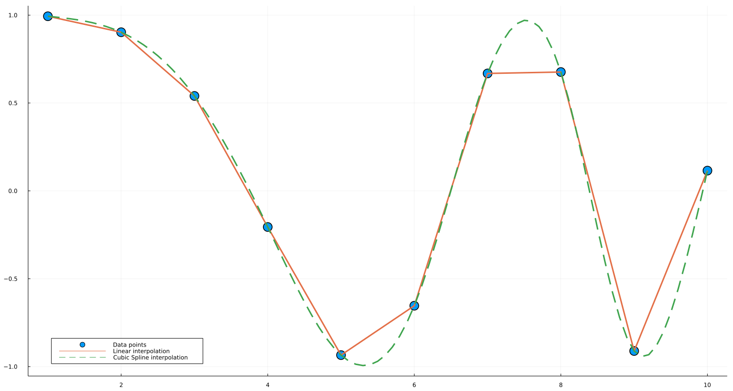
interp_linear_extrap(0.9) # outside grid: linear extrapolation

Other Examples

More examples, such as plotting and cubic interpolation, can be found at the convenience constructions documentation.

Performance shootout

In the perf directory, you can find a script that tests interpolation with several different packages. We consider interpolation in 1, 2, 3, and 4 dimensions, with orders 0 (Constant), 1 (Linear), and 2 (Quadratic). Methods include Interpolations BSpline (IBSpline) and Gridded (IGridded), methods from the Grid.jl package, methods from the Dierckx.jl package, methods from the GridInterpolations.jl package (GI), methods from the ApproXD.jl package, and methods from SciPy's RegularGridInterpolator accessed via PyCall (Py). All methods are tested using an Array with approximately 10^6 elements, and the interpolation task is simply to visit each grid point.

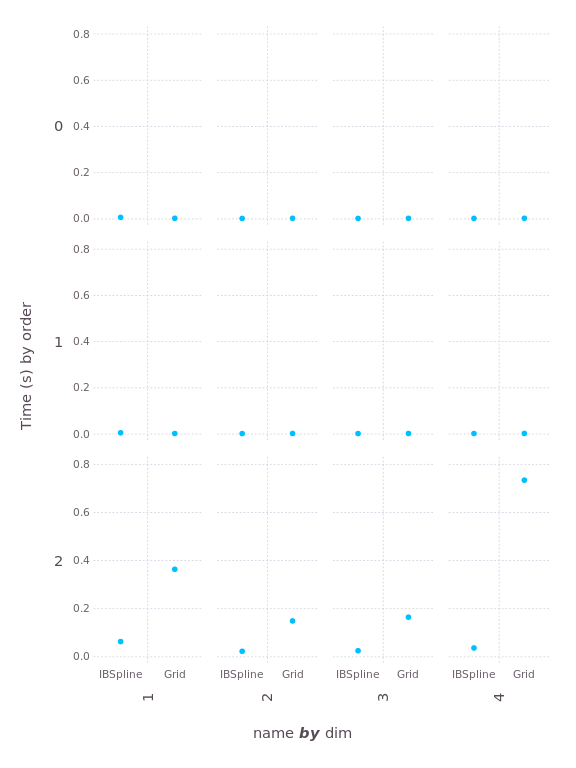
First, let's look at the two B-spline algorithms, IBspline and Grid. Here's a plot of the "construction time," the amount of time it takes to initialize an interpolation object (smaller is better):

The construction time is negligible until you get to second order (quadratic); that's because quadratic is the lowest order requiring the solution of tridiagonal systems upon construction. The solvers used by Interpolations are much faster than the approach taken in Grid.

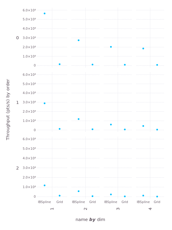
Now let's examine the interpolation performance. Here we'll measure "throughput", the number of interpolations performed per second (larger is better):

Once again, Interpolations wins on every test, by a factor that ranges from 7 to 13.

Now let's look at the "gridded" methods that allow irregular spacing along each axis. For some of these, we compare interpolation performance in both "vectorized" form itp[xvector, yvector] and in "scalar" form for y in yvector, x in xvector; val = itp[x,y]; end.

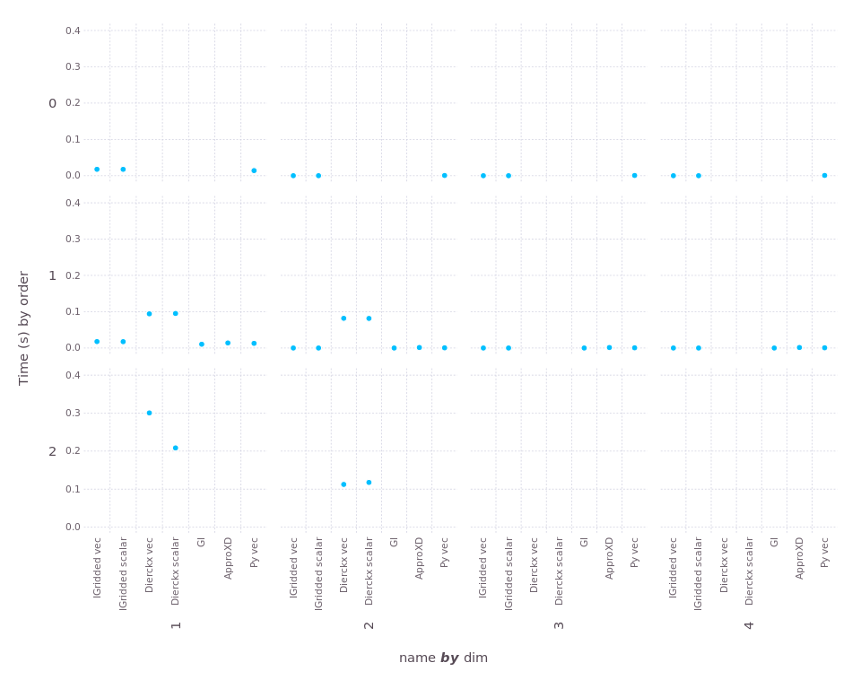
First, construction time (smaller is better):

Missing dots indicate cases that were not tested, or not supported by the package. (For construction, differences between "vec" and "scalar" are just noise, since no interpolation is performed during construction.) The only package that takes appreciable construction time is Dierckx.

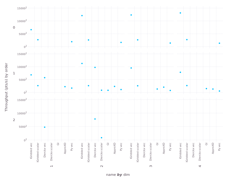
And here's "throughput" (larger is better). To ensure we can see the wide range of scales, here we use "square-root" scaling of the y-axis:

For 1d, the "Dierckx scalar" and "GI" tests were interrupted because they ran more than 20 seconds (far longer than any other test). Both performed much better in 2d, interestingly. You can see that Interpolations wins in every case, sometimes by a very large margin.

Contributing

Work is very much in progress, but help is always welcome. If you want to help out but don't know where to start, take a look at issue #5 - our feature wishlist =) There is also some developer documentation that may help you understand how things work internally.