RingsPy

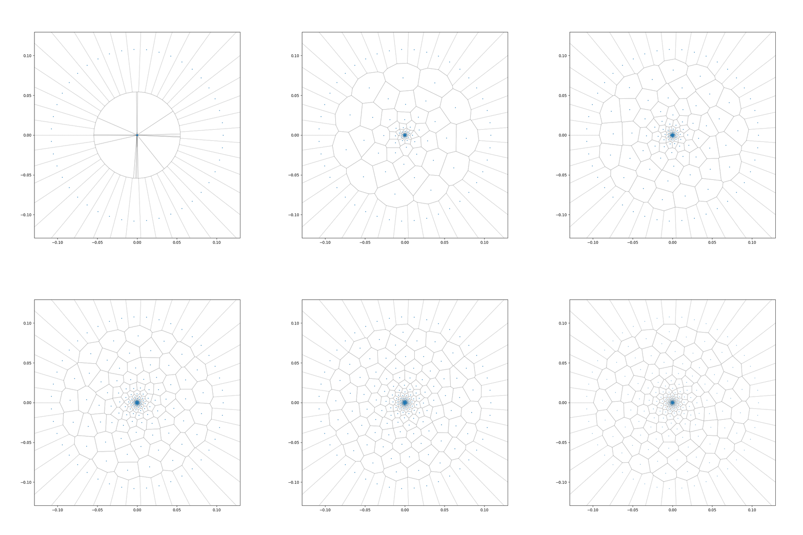
RingsPy is a Voronoi diagrams-based geometric generation tool that generates 3D meshes and models of prismatic cellular solids with radial growth rules.

Dependencies and Installation

RingsPy depends on mainstream Python libraries numpy and scipy, and optionally depends on library hexalattice, if a regular hexagonal lattice (e.g. honeycomb) is wanted; also vtk, if the 3D model files are also wanted.

1. pip install

To install RingsPy, one may use pip:

pip install ringspy

or use:

pip install git+https://github.com/kingyin3613/ringspy.git

to get updates beyond the latest release.

2. conda install

To install RingsPy in conda environments, one can also use conda-forge channel:

conda install -c conda-forge ringspy

3. Installation Check

There are some unit tests in tests. One can use pytest to check whether the installation is successful by firstly moving to ringspy or ringspy/tests directory and then running this command:

pytest .

Getting Started (Current version: v1.0.2)

Once all required components are installed and one is ready to begin, a path forward should be established for generating the mesh. The basic steps for running/viewing a cellular mesh are listed as the following:

1. Edit geometry and algorithm parameters
2. Generate mesh using Mesh Generation Tools
3. Visualize 2D view using Matplotlib or 3D model in `ParaView`
4. (Optional) Export 3D STL model for 3D editing and/or printing
5. (Optional) Export input file for numerical simulations with software `Abaqus`

1. Geometry and Parameters

The first step to generate a cellular geometry is selecting geometry and appropriate parameters.

1.1. Geometry

A template file, for example, test_wood_cube.py located in the tests directory acts as both the parameter input file, and main executable for the generation of a cubic wood specimen.

Note: The Mesh Generation Tool by now only accepts many of pre-defined boundary geometries (for v1.0.x, the following 3 shapes are supported: triangle, square, hexagon), importing of CAD and/or other 3D model files will be implemented in subsequent versions.

Note: for greatest compatibility create the geometry using all millimeters.

1.2. Parameters

By opening a input file, e.g., tests/test_wood_cube.py in any text editor, a file format similar to what is shown below will be displayed:

geoName = 'wood_cube'
path = 'meshes'

radial_growth_rule = 'binary'
iter_max = 500 # increase this number to achieve a more regular geometry
print_interval = 500 # interval for printing prgress info

# Radial cell growth parameters
# length unit: mm
r_min = 0   # inner radius of generation domain
r_max = 4   # outer radius of generation domain
nrings = 4 # number of rings
width_heart = 0.3*(r_max-r_min)/nrings # ring width for the innermost ring
width_sparse = 0.7*(r_max-r_min)/nrings # ring width for rings with sparse cells
width_dense = 0.3*(r_max-r_min)/nrings # ring width for rings with dense cells
generation_center = (0,0) # coordinates of generation domain center

cellsize_sparse = 0.02
cellsize_dense = 0.01
cellwallthickness_sparse = 0.010
cellwallthickness_dense = 0.006

# clipping box parameters
boundaryFlag = 'on'
box_shape = 'square'
box_center = (0,0) # coordinates of clipping box center
box_size = 4.0 # side length
	
# longitudinal direction parameters
nsegments = 2 # increase this number to achieve a smoother transition in longitudinal direction if theta is large
theta_min = 0 # unit: radian
theta_max = 0.05 # unit: radian
z_min = 0
z_max = box_size # segment_length = (z_max - z_min) / nsegments
long_connector_ratio = 0.02 # longitudinal joint length = ratio * segment_length

# material parameters
skeleton_density = 1.5e-9 # unit: tonne/mm3

# generation parameters
merge_operation = 'on'
merge_tol = 0.01

precrackFlag = 'off'
precrack_widths = 0.1

stlFlag = 'on'

inpFlag = 'on'
inpType = 'Abaqus'

geoName is the geometry name, path is the folder where the mesh files will be generated.
radial_growth_rule is the radial growth rule for cell placement. When a file name with extension.npy is specified, a saved cell data file will be loaded (for v1.0.x, choose one of these rules: binary, binary_lloyd, regular_hexagonal, or a file name with extension .npy).
iter_max is the max number of iteration for randomly placing non-overlapping cell particles in the 2D toroidal cell placement region. Noticing that, larger iter_max leads to more centroidal Voronoi cells, for more reference, see Wiki - Centroidal Voronoi Tessellation.
print_interval is the print interval when every n cell particles are placed in the placement region.
r_min and r_max are the upper and lower bounds of radii of toroidal cell placement regions (generation rings), nrings is the total number of rings.
width_heart, width_sparse, and width_dense, are ring widths for innermost ring, rings with sparse cells, and rings with dense cells, respectively, which all together determine the morphology of the cellular structure.
generation_center is the location of the placement region.
cellsize_sparse,cellsize_dense, cellwallthickness_sparse, and cellwallthickness_dense are parameters for the sparse and dense cells.
boundaryFlag flag can be turned on/off for generating neat boundaries consisting of grains.
box_shape is the shape of cutting box (for v1.0.x, choose one of following shapes: triangle, square, or hexagon).
box_center, and box_size are for describing the cutting box.
nsegments is the number of segments consisting the prismatic cells during the z- (longitudinal) extrusion, with segment_length = (z_max - z_min) / nsegments.
theta_min and theta_max determine the twisting angles (unit: radian) of the 2D mesh around the generation_center, during the spiral z-extrusion.
z_min and z_max determine the boundaries of prismatic cells in z- (longitudinal) direction.
long_connector_ratio is the length of longitudinal joints, with longitudinal joint length = ratio * segment_length.
skeleton_density is the density of the skeleton (substance) material, e.g. density of wood cell walls in the wood microstructure.
merge_operation flag can be turned on/off for the merging operation, when flag is on, cell ridges that are shorter than the threshold merge_tol in the 2D mesh will be deleted, and their vertices will be merged respectively, the mesh will be reconstructed. This is designed for eliminating small cell ridges/walls which fall out of the resolution range of the 3D printing and for avoiding having elements with too small stable time increments in numerical simulations.
precrackFlag flag is for inserting a pre-crack, for the notched specimens (for v1.0.x, only a single line pre-crack with the length of precrack_widths is supported).
stlFlag flag can be turned on/off for generating 3D STL files.
inpFlag flag can be turned on/off for generating input files for numerical simulations.
inpType indicates the software(s) that the mesh generation should generate input files for.

2.1. Run Mesh Generation

Open a Command Prompt or Terminal window and set the current directory to tests or any other directory, then run the command:

python test_wood_cube.py

Functions in MeshGenTools library will be called to create the initial mesh, wood cell particles following certain cell size distribution will be placed, then Scipy.voronoi function will be called to form the initial 2D Voronoi tessellation, additional code reforms the tesselation and generates the desired files. A successful generation will end with the line "Files generated ..." in the Terminal window.

A new folder should have been created in the .\meshes directory with the same name as the geoName in test_wood_cube.py.

${\textbf{(New feature in version v0.4.x)}}$

The Lloyd's relaxation (a.k.a. Lloyd's algorithm) has been integrated with the mesh generation, one may use this approach by changing the following line in the input file:

radial_growth_rule = binary_lloyd

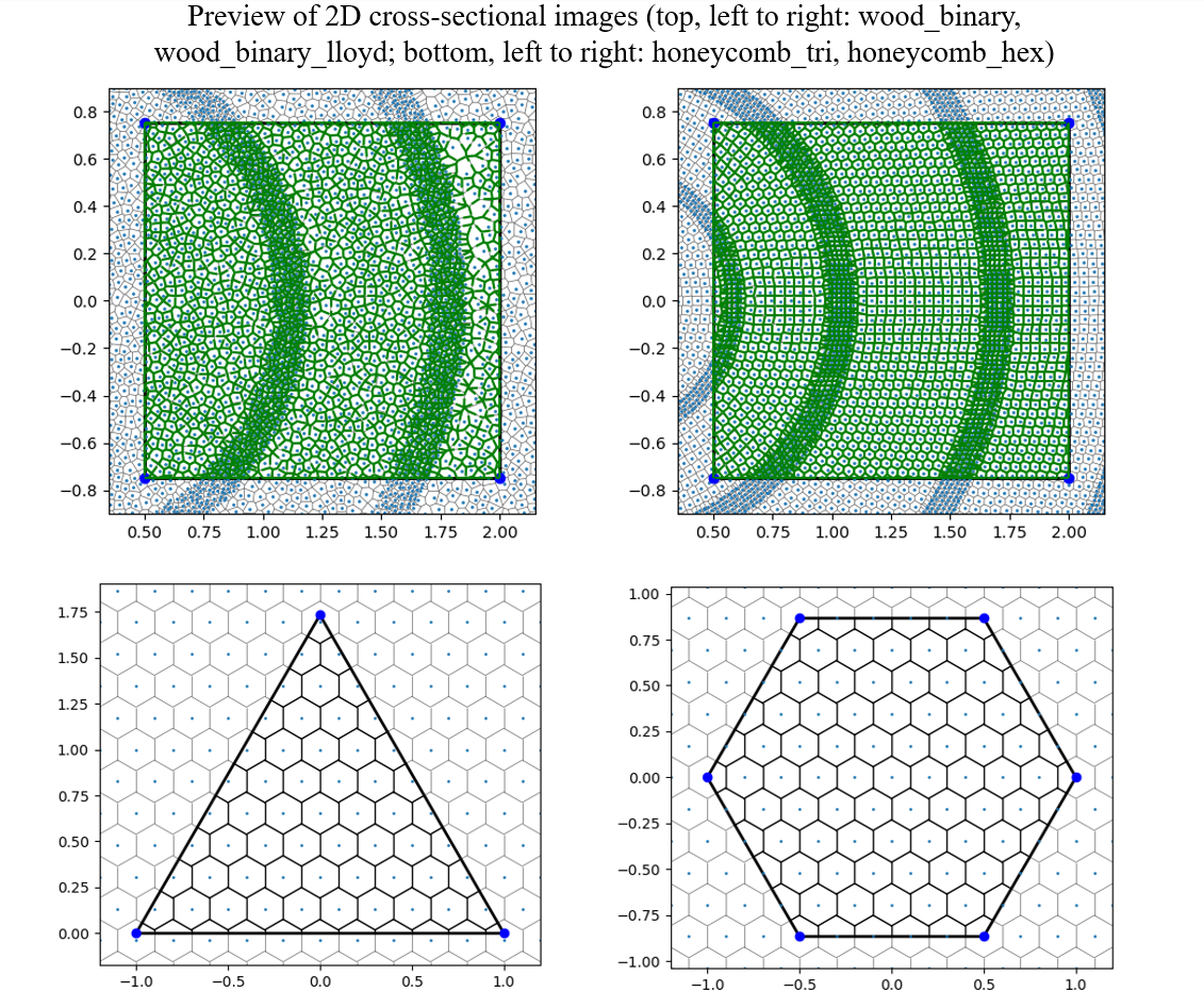
This allows a rapid radial generation of more regular centroidal Voronoi cells from the generation_center (see the difference between wood_binary and wood_binary_lloyd in the preview of 2D cross-sections in section 2.2). For more detail of the algorithm, see Wiki - Lloyd's algorithm).

2.2. Check Mesh and 3D Model Files

The following files should be generated in the .\meshes\geoName directory with a successful run:

Log file
- Log file for model generation: wood_cube-report.log
Mesh files
- Non-Uniform Rational B-Splines (NURBS) beam file: wood_cubeIGA.txt
- connector data file: wood_cube-mesh.txt
- Grain-ridge data file: wood_cube-vertex.mesh
- Ridge data file: wood_cube-ridge.mesh
Visualization files
- Cross-sectional image file for initial 2D configuration: wood_cube.png
- Paraview vtk file for initial vertex configuration: wood_cube_vertices.vtu
- Paraview vtk file for initial grain solid configuration: wood_cube_beams.vtu
- Paraview vtk file of initial cell ridge configuration: wood_cube_conns.vtu
- Paraview vtk file of initial connector (volume) configuration: wood_cube_conns_vol.vtu
(Optional) 3D model files
- STL file of initial cellular solid configuration: wood_cube.stl
(Optional) Abaqus input files
- INP file of simulation input of initial cellular solid configuration in Abaqus: wood_cube.inp

3. Visualization

A scientific visualization application ParaView can directly visualize the generated vtk files; It can also visualize generated 3D model STL files if the STL flag is on. Paraview is a free software, it can be downloaded from its official website: https://www.paraview.org/download/, latest version is recommeded.

3.1. Visualize Components of the 3D Model in ParaView

1. Open ParaView
2. Recommeded to temporarily turn off ray tracing
    - Uncheck "Enable Ray Tracing" (bottom left)
3. Open File Sets in `.\meshes\geoName`
    - File > Open...
4. Select the visualization files containing: `_vertices.vtu`, `_beams.vtu`, `_conns.vtu`
5. Apply to visualize
    - Press Apply (left side, center)
6. Turn on color plotting
    - Left click `_conns.vtu`, then select coloring (mid/lower left) > Connector_width
7. Scale and position the image as desired
8. Turn back on Ray Tracing
9. Adjust Ray Tracing lighting and settings as desired
10. Export Image
    - File > Save Screenshot
    - Enter a file name > OK
    - Leave new window as-is or increase resolution > OK

3.2. Visualize Volumes of the 3D Model in ParaView

1. Open Paraview
2. Recommeded to temporarily turn off ray tracing
    - Uncheck "Enable Ray Tracing" (bottom left)
3. Open File Sets in `.\meshes\geoName`
    - File > Open...
4. Select the newly created visualization files containing: `_conns_vol.vtu`
5. Apply to visualize
    - Press Apply (left side, center)
6. Turn on color plotting
    - Left click `_conns_vol.vtu`, then select coloring (mid/lower left) > Connector_width
7. Scale and position the image as desired
8. Turn back on Ray Tracing
9. Adjust Ray Tracing lighting and settings as desired
10. Export Image
    - File > Save Screenshot
    - Enter a file name > OK
    - Leave new window as-is or increase resolution > OK

4. (Optional) Numerical Simulation

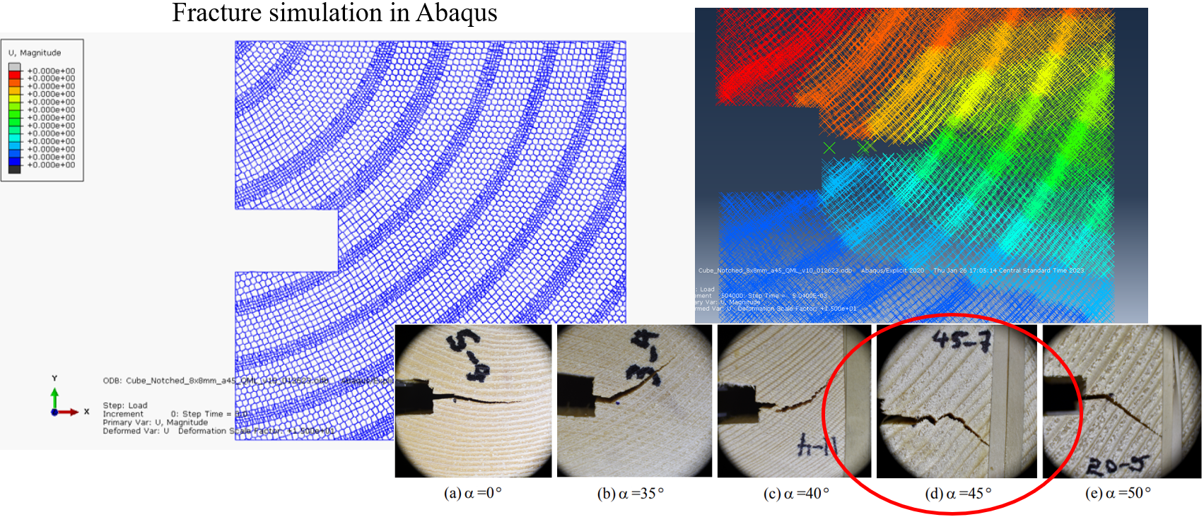
The mesh generation tool can also prepare the input files for the numerical simulations of the cellular solid in other softwares. By now (version 1.0.x), the input file format, .inp, that is used in a finite element method (FEM) software Abaqus is supported, if the INP flag is on. Abaqus is a commerical software suite for integrated computer-aided engineering (CAE) and finite element analysis, own by Dassault Systèmes. One may refer to its Wiki for more about Abaqus, and to Introduction for the introduction of Abaqus input files.

All steps for the model setup can be accomplished through manually coding the Abaqus input file in a text editor. The method used in the example procedure shown below requires access to the Abaqus GUI.

4.1 Create New Model

1. Open Abaqus CAE
2. Create a new model
    -	File > New Model Database > With Standard/Explicit Model

4.2 Import Meshed Part

1. Import the meshed part
    - File > Import > Part
    - Select the newly created file which ends in `.inp` (note: you may need to change the File Filter to see this file)
    - Click OK
2. Rename part
    - Under the model tree (left) expand `Parts`
    - Right click on the part > Rename...
    - Enter a new name less than 14 characters, no special symbols, and easily recognizable (i.e. "WoodCube")

Note: if FEM parts will be added to the model, this RingsPy generated part must come first alphabetically. Also recommended not to include numbers in the name.

Contributing

If you make use of this code, or find it is useful for your own research , please cite the JOSS paper:

@article{ringspy,
    doi = {10.21105/joss.04945},
    url = {https://doi.org/10.21105/joss.04945},
    year = {2023},
    publisher = {The Open Journal},
    volume = {8},
    number = {83},
    pages = {4945},
    author = {Hao Yin and Gianluca Cusatis},
    title = {RingsPy: A Python package for Voronoi mesh generation of cellular solids with radial growth pattern},
    journal = {Journal of Open Source Software}
}

Contributions are always welcome!

If you wish to contribute code/algorithms to this project, or to propose a collaboration study, please send an email to haoyin2022 [at] u.northwestern.edu .

tianjuchen/ringspy