An implementation of the FASSTER (Forecasting with Additive Switching of Seasonality, Trend and Exogenous Regressors) model in R. This model is designed to capture patterns of multiple seasonality in a state space framework by using state switching. The fasster package prioritizes flexibility, computational speed and accuracy to provide convenient tools for modelling, predicting and understanding high frequency time-series.
This package is early in development, and there are plans to make substantial changes in the future.
The latest usage examples of using fasster can be found in my useR! 2018 talk: slides, video, source.
There are further plans to improve the heuristic optimisation techniques and better use sparse matrix algebra (removing the dlm package dependency) to make fasster even faster. Implementing this will likely result in a revision of the model object structure, but user directed functionality should remain the same.
The development version can be installed from GitHub using:
# install.packages("devtools")
devtools::install_github("tidyverts/fasster")fasster allows flexible model specification by allowing the user to specify the model structure with standard formula conventions.
library(fasster)
library(tidyverse)
library(lubridate)
library(tsibble)
library(fable)

lung_deaths <- as_tsibble(cbind(mdeaths, fdeaths), pivot_longer = FALSE)
fit <- lung_deaths %>%
  model(fasster = FASSTER(fdeaths ~ mdeaths))
fit %>% report()
#> Series: fdeaths
#> Model: FASSTER
#>
#> Estimated variances:
#>  State noise variances (W):
#>   mdeaths
#>    1.7119e-34
#>
#>  Observation noise variance (V):
#>   1.6631e+03
Commonly used state space components can be added using the following convenience functions:
trend(n)to include an n-th order polynomialseason(s)to include a seasonal factor of frequency sfourier(s, q)to include seasonal fourier terms of frequency s with q harmonicsarma(ar, ma)to include an ARMA term (where ar and ma are vectors of coefficients)- Exogenous regressors can be added by referring to their name
For example, to create a model with trend and monthly seasonality, you can use:
fit <- as_tsibble(USAccDeaths) %>%
  model(fasster = FASSTER(value ~ trend(1) + fourier(12)))
fit %>% report()
#> Series: value
#> Model: FASSTER
#>
#> Estimated variances:
#>  State noise variances (W):
#>   fourier(12)
#>    6.6663e-13 7.5474e-13 3.6532e-13 3.6933e-13 3.3369e-13 2.8588e-13 4.2485e-13 2.2424e-13 3.2003e-13 2.1307e-13 1.8887e-13
#>   trend(1)
#>    5.9382e+03
#>
#>  Observation noise variance (V):
#>   2.0543e+04
The interface for creating a FASSTER model introduces a new formula
construct, %S%, known as the switch operator. This allows modelling of
more complex patterns such as multiple seasonality by modelling the
components for each group separately and switching between them.
elec_tr <- tsibbledata::vic_elec %>%
  filter(
    Time < lubridate::ymd("2012-03-01")
  ) %>%
  mutate(WorkDay = wday(Time) %in% 2:6 & !Holiday)

elec_fit <- elec_tr %>%
  model(
    fasster = fasster(log(Demand) ~
      WorkDay %S% (fourier(48, 16) + trend(1)) + Temperature + I(Temperature^2)
    )
)Fitted FASSTER models can be decomposed to provide a description of how the underlying states function. Decomposing a FASSTER model provides aggregates of its components such as trends and seasonalities.
These components can accessed from a fitted model using the
components() function:
fit %>%
  components()
#> # A dable:               72 x 5 [1M]
#> # Key:                   .model [1]
#> # FASSTER Decomposition: value = `fourier(12)` + `trend(1)`
#>    .model     index value `fourier(12)` `trend(1)`
#>    <chr>      <mth> <dbl>         <dbl>      <dbl>
#>  1 fasster 1973 Jan  9007        -795.       9740.
#>  2 fasster 1973 Feb  8106       -1546.       9754.
#>  3 fasster 1973 Mar  8928        -758.       9719.
#>  4 fasster 1973 Apr  9137        -536.       9706.
#>  5 fasster 1973 May 10017         322.       9693.
#>  6 fasster 1973 Jun 10826         802.       9694.
#>  7 fasster 1973 Jul 11317        1669.       9830.
#>  8 fasster 1973 Aug 10744         974.       9755.
#>  9 fasster 1973 Sep  9713         -65.7      9761.
#> 10 fasster 1973 Oct  9938         233.       9768.
#> # … with 62 more rows
elec_fit %>%
components()
#> # A dable: 2,880 x 9 [30m] <Australia/Melbourne>
#> # Key: .model [1]
#> # FASSTER Decomposition: log(Demand) = `WorkDay_FALSE/fourier(48, 16)` +
#> # `WorkDay_FALSE/trend(1)` + `WorkDay_TRUE/fourier(48, 16)` +
#> # `WorkDay_TRUE/trend(1)` + Temperature + `I(Temperature^2)`
#> .model Time `log(Demand)` `WorkDay_FALSE/… `WorkDay_FALSE/…
#> <chr> <dttm> <dbl> <dbl> <dbl>
#> 1 fasst… 2012-01-01 00:00:00 8.39 -0.00345 8.75
#> 2 fasst… 2012-01-01 00:30:00 8.36 -0.0234 8.75
#> 3 fasst… 2012-01-01 01:00:00 8.31 -0.0971 8.75
#> 4 fasst… 2012-01-01 01:30:00 8.26 -0.105 8.76
#> 5 fasst… 2012-01-01 02:00:00 8.30 -0.117 8.76
#> 6 fasst… 2012-01-01 02:30:00 8.26 -0.0812 8.78
#> 7 fasst… 2012-01-01 03:00:00 8.21 -0.251 8.76
#> 8 fasst… 2012-01-01 03:30:00 8.18 -0.144 8.82
#> 9 fasst… 2012-01-01 04:00:00 8.14 -0.374 8.68
#> 10 fasst… 2012-01-01 04:30:00 8.12 -0.202 8.81
#> # … with 2,870 more rows, and 4 more variables: `WorkDay_TRUE/fourier(48,
#> # 16)` <dbl>, `WorkDay_TRUE/trend(1)` <dbl>, Temperature <dbl>,
#> # `I(Temperature^2)` <dbl>The tools made available by fasster are designed to integrate seamlessly with the tidyverse of packages, enabling familiar data manipulation and visualisation capabilities.
fasster conforms to the object structure from the fable package, allowing common visualisation and analysis tools to be applied on FASSTER models.
fit %>%
  forecast(h=24) %>%
  autoplot(as_tsibble(USAccDeaths))
Future index values are automatically produced and used where necessary
in the model specification. If additional information is required by the
model (such as WorkDay and Temperature) they must be included in a
tsibble of future values passed to new_data.
elec_ts <- tsibbledata::vic_elec %>%
  filter(
    yearmonth(Time) == yearmonth("2012 Mar")
  ) %>%
  mutate(WorkDay = wday(Time) %in% 2:6 & !Holiday) %>%
  select(-Demand)
elec_fit %>%
  forecast(new_data = elec_ts) %>%
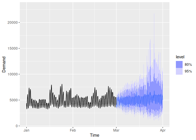
  autoplot(elec_tr)
Please note that this project is released with a Contributor Code of Conduct. By participating in this project you agree to abide by its terms.


