This repository contains the details and references for all NLP topics. Below is the list of topics:
- TF-IDF
- Conditional Random Field
- Word Embeddings
- Recurrent Neural Network
- LSTM
- ELMO
- Flair
- ULMFIT
- Attention
- Transformer
- BERT
- BERT limitations
- ALBERT
- DistilBERT
- ROBERTA
- XLNET
- Sentence BERT
- GPT-1
- GPT-2
- GPT-3
- ChatGPT
- Prompt Engineering
- Choosing the right LM for your usecase
- TF-IDF (term frequency-inverse document frequency) is a statistical measure that evaluates how relevant a word is to a document in a collection of documents.
- This is done by multiplying two metrics: how many times a word appears in a document, and the inverse document frequency of the word across a set of documents.
- TF-IDF was invented for document search and information retrieval. It works by increasing proportionally to the number of times a word appears in a document, but is offset by the number of documents that contain the word. So, words that are common in every document, such as this, what, and if, rank low even though they may appear many times, since they don’t mean much to that document in particular.
- However, if the word Bug appears many times in a document, while not appearing many times in others, it probably means that it’s very relevant. For example, if what we’re doing is trying to find out which topics some NPS responses belong to, the word Bug would probably end up being tied to the topic Reliability, since most responses containing that word would be about that topic.
- How is TF-IDF calculated?
- TF-IDF for a word in a document is calculated by multiplying two different metrics:
- The term frequency of a word in a document. There are several ways of calculating this frequency, with the simplest being a raw count of instances a word appears in a document. Then, there are ways to adjust the frequency, by length of a document, or by the raw frequency of the most frequent word in a document.
- The inverse document frequency of the word across a set of documents. This means, how common or rare a word is in the entire document set. The closer it is to 0, the more common a word is. This metric can be calculated by taking the total number of documents, dividing it by the number of documents that contain a word, and calculating the logarithm.
- So, if the word is very common and appears in many documents, this number will approach 0. Otherwise, it will approach 1.
- Multiplying these two numbers results in the TF-IDF score of a word in a document. The higher the score, the more relevant that word is in that particular document.
- The TF-IDF score for the word t in the document d from the document set D is calculated as follows: tf_idf(t,d,D) = tf(t,d)*idf(t,D) where tf(t,d) = log(1+freq(t,d)) idf(t,D) = log(N/count(d belongs to D: t belongs to d))
- TF-IDF for a word in a document is calculated by multiplying two different metrics:
- References:
- Conditional Random Fields are a discriminative model, used for predicting sequences. They use contextual information from previous labels, thus increasing the amount of information the model has to make a good prediction.
- Part of speech tagging:
-
Let’s go into some more detail, using the more common example of part-of-speech tagging. In POS tagging, the goal is to label a sentence (a sequence of words or tokens) with tags like ADJECTIVE, NOUN, PREPOSITION, VERB, ADVERB, ARTICLE. For example, given the sentence “Bob drank coffee at Starbucks”, the labeling might be “Bob (NOUN) drank (VERB) coffee (NOUN) at (PREPOSITION) Starbucks (NOUN)”. So let’s build a conditional random field to label sentences with their parts of speech. Just like any classifier, we’ll first need to decide on a set of feature functions fi.
-
Feature Functions in a CRF
- In a CRF, each feature function is a function that takes in as input:
- a sentence s
- the position i of a word in the sentence
- the label li of the current word
- the label li−1 of the previous word and outputs a real-valued number (though the numbers are often just either 0 or 1). Note: by restricting our features to depend on only the current and previous labels, rather than arbitrary labels throughout the sentence, I’m actually building the special case of a linear-chain CRF.
- In a CRF, each feature function is a function that takes in as input:
-
Features to Probabilities
- Next, assign each feature function fj a weight λj (I’ll talk below about how to learn these weights from the data). Given a sentence s, we can now score a labeling l of s by adding up the weighted features over all words in the sentence:
$$score(l/s) =\sum_{j=1}^m \sum_{i=1}^n λ_jf_j(s,i,l_i,l_{i-1})$$
(The first sum runs over each feature function j, and the inner sum runs over each position i of the sentence.)
Finally, we can transform these scores into probabilities p(l|s) between 0 and 1 by exponentiating and normalizing: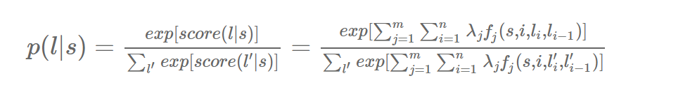
- Next, assign each feature function fj a weight λj (I’ll talk below about how to learn these weights from the data). Given a sentence s, we can now score a labeling l of s by adding up the weighted features over all words in the sentence:
-
Example Feature Functions
So what do these feature functions look like? Examples of POS tagging features could include:-
$$f1(s,i,l_i,l_{i−1})=1$$ if li= ADVERB and the ith word ends in “-ly”; 0 otherwise. ** If the weight λ1 associated with this feature is large and positive, then this feature is essentially saying that we prefer labelings where words ending in -ly get labeled as ADVERB. -
$$f2(s,i,l_i,l_{i−1})=1$$ if i=1, li= VERB, and the sentence ends in a question mark; 0 otherwise. ** Again, if the weight λ2 associated with this feature is large and positive, then labelings that assign VERB to the first word in a question (e.g., “Is this a sentence beginning with a verb?”) are preferred. -
$$f3(s,i,l_i,l_{i−1})=1$$ if li-1= ADJECTIVE and li= NOUN; 0 otherwise. ** Again, a positive weight for this feature means that adjectives tend to be followed by nouns. -
$$f4(s,i,l_i,l_{i−1})=1$$ if li−1= PREPOSITION and li= PREPOSITION. ** A negative weight λ4 for this function would mean that prepositions don’t tend to follow prepositions, so we should avoid labelings where this happens.
And that’s it! To sum up: to build a conditional random field, you just define a bunch of feature functions (which can depend on the entire sentence, a current position, and nearby labels), assign them weights, and add them all together, transforming at the end to a probability if necessary.
-
-
Learning Weights: Let’s go back to the question of how to learn the feature weights in a CRF. One way, unsurprisingly, is to use gradient descent.
Assume we have a bunch of training examples (sentences and associated part-of-speech labels). Randomly initialize the weights of our CRF model. To shift these randomly initialized weights to the correct ones, for each training example…- Go through each feature function fi, and calculate the gradient of the log probability of the training example with respect to

- Note that the first term in the gradient is the contribution of feature fi under the true label, and the second term in the gradient is the expected contribution of feature fi under the current model. This is exactly the form you’d expect gradient ascent to take.
- Move λi in the direction of the gradient:

where α is some learning rate. - Repeat the previous steps until some stopping condition is reached (e.g., the updates fall below some threshold).
- Go through each feature function fi, and calculate the gradient of the log probability of the training example with respect to
-
Finding the Optimal Labeling: Suppose we’ve trained our CRF model, and now a new sentence comes in. How do we do label it?
The naive way is to calculate p(l|s) for every possible labeling l, and then choose the label that maximizes this probability. However, since there are km possible labels for a tag set of size k and a sentence of length m, this approach would have to check an exponential number of labels.
A better way is to realize that (linear-chain) CRFs satisfy an optimal substructure property that allows us to use a (polynomial-time) dynamic programming algorithm to find the optimal label, similar to the Viterbi algorithm for HMMs.
-
- References:


Word embeddings are a type of word representation that allows words with similar meaning to have a similar representation. Word embeddings help in generating the distributed representation for text which are lower in dimension as compare to other text representation techniques like TF-IDF. One of the benefits of using dense and low-dimensional vectors is computational: the majority of neural network toolkits do not play well with very high-dimensional, sparse vectors. … The main benefit of the dense representations is generalization power: if we believe some features may provide similar clues, it is worthwhile to provide a representation that is able to capture these similarities.
- Word2Vec uses a trick in which we train a simple neural network with a single hidden layer to perform a certain task, but then we’re not actually going to use that neural network for the task we trained. nstead, the goal is actually just to learn the weights of the hidden layer–we’ll see that these weights are actually the “word vectors” that we’re trying to learn.
- The Fake task: Given a specific word in the middle of a sentence (the input word), look at the words nearby and pick one at random. The network is going to tell us the probability for every word in our vocabulary of being the “nearby word” that we chose. Here, "nearby" means there is actually a "window size" parameter to the algorithm. A typical window size might be 5, meaning 5 words behind and 5 words ahead (10 in total). The output probabilities are going to relate to how likely it is find each vocabulary word nearby our input word. For example, if you gave the trained network the input word “Soviet”, the output probabilities are going to be much higher for words like “Union” and “Russia” than for unrelated words like “watermelon” and “kangaroo”.
- We’ll train the neural network to do this by feeding it word pairs found in our training documents. The below example shows some of the training samples (word pairs) we would take from the sentence “The quick brown fox jumps over the lazy dog.” I’ve used a small window size of 2 just for the example. The word highlighted in blue is the input word.

The network is going to learn the statistics from the number of times each pairing shows up. So, for example, the network is probably going to get many more training samples of (“Soviet”, “Union”) than it is of (“Soviet”, “Sasquatch”). When the training is finished, if you give it the word “Soviet” as input, then it will output a much higher probability for “Union” or “Russia” than it will for “Sasquatch”. - Model Details

The above is the architecture of 1 hidden layer neural network. - Let's consider we have 10,000 uinque words in the vocab. Here we represent any input work like "machine" as a one-hot vector. The output of the network is a single vector (also with 10,000 components) containing, for every word in our vocabulary, the probability that a randomly selected nearby word is that vocabulary word. There is no activation function on the hidden layer neurons, but the output neurons use softmax.
- When training this network on word pairs, the input is a one-hot vector representing the input word and the training output is also a one-hot vector representing the output word. But when you evaluate the trained network on an input word, the output vector will actually be a probability distribution (i.e., a bunch of floating point values, not a one-hot vector).
- Hidden Layer
- Let's say we are trying to learn word vectors with 300 dimension. So the hidden layer is going to be represented by a weight matrix with 10,000 rows (one for every word in our vocabulary) and 300 columns (one for every hidden neuron). If you look at the rows of this weight matrix, these are actually what will be our word vectors!

So the end goal of all of this is really just to learn this hidden layer weight matrix – the output layer we’ll just toss when we’re done!. Here the hidden layer of this model is really just operating as a lookup table. The output of the hidden layer is just the “word vector” for the input word.
- Let's say we are trying to learn word vectors with 300 dimension. So the hidden layer is going to be represented by a weight matrix with 10,000 rows (one for every word in our vocabulary) and 300 columns (one for every hidden neuron). If you look at the rows of this weight matrix, these are actually what will be our word vectors!
- Output layer
- The 1 x 300 word vector for “machine” then gets fed to the output layer. The output layer is a softmax regression classifier. Each output neuron (one per word in our vocabulary!) will produce an output between 0 and 1, and the sum of all these output values will add up to 1. Specifically, each output neuron has a weight vector which it multiplies against the word vector from the hidden layer, then it applies the function exp(x) to the result. Finally, in order to get the outputs to sum up to 1, we divide this result by the sum of the results from all 10,000 output nodes.
- Intuition
- If two different words have very similar “contexts” (that is, what words are likely to appear around them), then our model needs to output very similar results for these two words. And one way for the network to output similar context predictions for these two words is if the word vectors are similar. So, if two words have similar contexts, then our network is motivated to learn similar word vectors for these two words. And what does it mean for two words to have similar contexts? I think you could expect that synonyms like “intelligent” and “smart” would have very similar contexts. Or that words that are related, like “engine” and “transmission”, would probably have similar contexts as well. This can also handle stemming for you – the network will likely learn similar word vectors for the words “ant” and “ants” because these should have similar contexts.
- References
- http://ruder.io/word-embeddings-softmax/index.html#noisecontrastiveestimation
- http://mccormickml.com/2016/04/19/word2vec-tutorial-the-skip-gram-model/
- http://mccormickml.com/2017/01/11/word2vec-tutorial-part-2-negative-sampling/
- https://machinelearningmastery.com/what-are-word-embeddings/
- http://jalammar.github.io/illustrated-word2vec/


GloVe stands for global vectors for word representation. Unlike Word2vec, GloVe does not rely just on local statistics (local context information of words), but incorporates global statistics (word co-occurrence) to obtain word vectors. It generates word embeddings by aggregating global word-word co-occurrence matrix from a corpus. It is an approach to marry both the global statistics of matrix factorization techniques like LSA (Latent Semantic Analysis) with the local context-based learning in word2vec. Rather than using a window to define local context, GloVe constructs an explicit word-context or word co-occurrence matrix using statistics across the whole text corpus.
THe GloVe algorithm consists of following steps:
- Collect word co-occurence statistics in a form of word co-ocurrence matrix X. Each element Xij of such matrix represents how often word i appears in context of word j. Usually we scan our corpus in the following manner: for each term we look for context terms within some area defined by a window_size before the term and a window_size after the term. Also we give less weight for more distant words, usually using this formula: decay=1/offset
- Define soft constraints for each word pair:

Here wi - vector for the main word, wj - vector for the context word, bi, bj are scalar biases for the main and context words. - Define a cost function

Here f is a weighting function which help us to prevent learning only from extremely common word pairs. The GloVe authors choose the following function:


- Details
RNN is a family of neural network models which is designed to model sequential data. The idea behind RNNs is to make use of sequential information. In a traditional neural network we assume that all inputs (and outputs) are independent of each other. But for many tasks that’s a bad idea. If you want to predict the next word in a sentence you better know which words came before it. RNNs are called recurrent because they perform the same task for every element of a sequence, with the output being depended on the previous computations. Another way to think about RNNs is that they have a “memory” which captures information about what has been calculated so far. In theory RNNs can make use of information in arbitrarily long sequences, but in practice they are limited to looking back a fixed number of steps (more on this later). Here is what a typical RNN looks like:

The above diagram shows an RNN being unrolled (or unfolded) into a full network. By unrolling we simply mean that we write out the network for the complete sequence. For example, if the sequence we care about is a sentence of 5 words, the network would be unrolled into a 5-layer neural network, one layer for each word. The formulas that govern the computation happening in a RNN are as follows:
- xt is the input at time step t. For example, x1 could be a one-hot vector corresponding to the second word of a sentence.
- st is the hidden state at time step t. It’s the “memory” of the network. st is calculated based on the previous hidden state and the input at the current step: st = f(Uxt + Wxt). The function ff usually is a nonlinearity such as tanh or ReLU. s-1, which is required to calculate the first hidden state, is typically initialized to all zeroes.
- ot is the output at step t. For example, if we wanted to predict the next word in a sentence it would be a vector of probabilities across our vocabulary. ot = softmax(Vst).
There are a few things to note here:- You can think of the hidden state st as the memory of the network. st captures information about what happened in all the previous time steps. The output at step ot is calculated solely based on the memory at time t. As briefly mentioned above, it’s a bit more complicated in practice because st typically can’t capture information from too many time steps ago.
- Unlike a traditional deep neural network, which uses different parameters at each layer, a RNN shares the same parameters (U,V,W) across all steps. This reflects the fact that we are performing the same task at each step, just with different inputs. This greatly reduces the total number of parameters we need to learn.
- The above diagram has outputs at each time step, but depending on the task this may not be necessary. For example, when predicting the sentiment of a sentence we may only care about the final output, not the sentiment after each word. Similarly, we may not need inputs at each time step. The main feature of an RNN is its hidden state, which captures some information about a sequence.
- Vanishing Gradient
In RNN, the information travels through time which means that information from previous time points is used as input for the next time points. Cost function calculation or error is done at each point of time. Basically, during the training, your cost function compares your outcomes (red circles on the image below) to your desired output. As a result, you have these values throughout the time series, for every single one of these red circles.

Let’s focus on one error term et. You’ve calculated the cost function et, and now you want to propagate your cost function back through the network because you need to update the weights. Essentially, every single neuron that participated in the calculation of the output, associated with this cost function, should have its weight updated in order to minimize that error. And the thing with RNNs is that it’s not just the neurons directly below this output layer that contributed but all of the neurons far back in time. So, you have to propagate all the way back through time to these neurons. The problem relates to updating wrec (weight recurring) – the weight that is used to connect the hidden layers to themselves in the unrolled temporal loop. For instance, to get from xt-3 to xt-2 we multiply xt-3 by wrec. Then, to get from xt-2 to xt-1 we again multiply xt-2 by wrec. So, we multiply with the same exact weight multiple times, and this is where the problem arises: when you multiply something by a small number, your value decreases very quickly. As we know, weights are assigned at the start of the neural network with the random values, which are close to zero, and from there the network trains them up. But, when you start with wrec close to zero and multiply xt, xt-1, xt-2, xt-3, … by this value, your gradient becomes less and less with each multiplication.
- What does this mean for the network? The lower the gradient is, the harder it is for the network to update the weights and the longer it takes to get to the final result. For instance, 1000 epochs might be enough to get the final weight for the time point t, but insufficient for training the weights for the time point t-3 due to a very low gradient at this point. However, the problem is not only that half of the network is not trained properly. The output of the earlier layers is used as the input for the further layers. Thus, the training for the time point t is happening all along based on inputs that are coming from untrained layers. So, because of the vanishing gradient, the whole network is not being trained properly. For the vanishing gradient problem, the further you go through the network, the lower your gradient is and the harder it is to train the weights, which has a domino effect on all of the further weights throughout the network.
- References:


- LSTMs are explicitly designed to avoid the long-term dependency problem or vanishing gradient problem. The key to LSTMs is the cell state, the horizontal line running through the top of the diagram. The cell state is kind of like a conveyor belt. It runs straight down the entire chain, with only some minor linear interactions. It’s very easy for information to just flow along it unchanged.

- The LSTM does have the ability to remove or add information to the cell state, carefully regulated by structures called gates. Gates are a way to optionally let information through. They are composed out of a sigmoid neural net layer and a pointwise multiplication operation. The sigmoid layer outputs numbers between zero and one, describing how much of each component should be let through. A value of zero means “let nothing through,” while a value of one means “let everything through!”. An LSTM has three of these gates, to protect and control the cell state.
- The first step in our LSTM is to decide what information we’re going to throw away from the cell state. This decision is made by a sigmoid layer called the “forget gate layer.” It looks at ht−1 and xt, and outputs a number between 0 and 1 for each number in the cell state Ct−1. A 1 represents “completely keep this” while a 0 represents “completely get rid of this.”
- Let’s go back to our example of a language model trying to predict the next word based on all the previous ones. In such a problem, the cell state might include the gender of the present subject, so that the correct pronouns can be used. When we see a new subject, we want to forget the gender of the old subject.

- The next step is to decide what new information we’re going to store in the cell state. This has two parts. First, a sigmoid layer called the “input gate layer” decides which values we’ll update. Next, a tanh layer creates a vector of new candidate values, C~t, that could be added to the state. In the next step, we’ll combine these two to create an update to the state. In the example of our language model, we’d want to add the gender of the new subject to the cell state, to replace the old one we’re forgetting.

- It’s now time to update the old cell state, Ct−1, into the new cell state Ct. The previous steps already decided what to do, we just need to actually do it.
We multiply the old state by ft, forgetting the things we decided to forget earlier. Then we add it∗C~t. This is the new candidate values, scaled by how much we decided to update each state value. In the case of the language model, this is where we’d actually drop the information about the old subject’s gender and add the new information, as we decided in the previous steps.

- Finally, we need to decide what we’re going to output. This output will be based on our cell state, but will be a filtered version. First, we run a sigmoid layer which decides what parts of the cell state we’re going to output. Then, we put the cell state through tanh (to push the values to be between −1 and 1) and multiply it by the output of the sigmoid gate, so that we only output the parts we decided to. For the language model example, since it just saw a subject, it might want to output information relevant to a verb, in case that’s what is coming next. For example, it might output whether the subject is singular or plural, so that we know what form a verb should be conjugated into if that’s what follows next.

- How LSTM solves vanishing gradient problem
- References:


ELMO achieves state-of-the-art performance on many popular tasks including question-answering, sentiment analysis, and named-entity extraction

ELMo word vectors are computed on top of a two-layer bidirectional language model (biLM). This biLM model has two layers stacked together. Each layer has 2 passes — forward pass and backward pass.
- The architecture above uses a character-level convolutional neural network (CNN) to represent words of a text string into raw word vectors
- These raw word vectors act as inputs to the first layer of biLM
- The forward pass contains information about a certain word and the context (other words) before that word
- The backward pass contains information about the word and the context after it
- This pair of information, from the forward and backward pass, forms the intermediate word vectors
- These intermediate word vectors are fed into the next layer of biLM
- The final representation (ELMo) is the weighted sum of the raw word vectors and the 2 intermediate word vectors As the input to the biLM is computed from characters rather than words, it captures the inner structure of the word. For example, the biLM will be able to figure out that terms like beauty and beautiful are related at some level without even looking at the context they often appear in. Sounds incredible! Unlike traditional word embeddings such as word2vec and GLoVe, the ELMo vector assigned to a token or word is actually a function of the entire sentence containing that word. Therefore, the same word can have different word vectors under different contexts.
- Elmo is open source
- It's code and datasets are open source. It has a website which includes not only basic information about it, but also download links for the small, medium, and original versions of the model. People looking to use ELMo should definitely check out this website to get a quick copy of the model. Moreover, the code is published on GitHub and includes a pretty-extensive README that lets users know how to use ELMo. I’d be surprised if it took anyone more than a few hours to get a working ELMo model going.
- Code: https://github.com/allenai/allennlp
- Website: https://allenai.org/allennlp/software/elmo
- References
FLAIR library provides powerful state-of-the-art contextual word embeddings. It provides following features:
- Flair supports a number of word embeddings used to perform NLP tasks such as FastText, ELMo, GloVe, BERT and its variants, XLM, and Byte Pair Embeddings including Flair Embedding.
- The Flair Embedding is based on the concept of contextual string embeddings which is used for Sequence Labelling.
- Using Flair you can also combine different word embeddings together to get better results.
Flair supports a number of languages.
In this word embedding each of the letters in the words are sent to the Character Language Model and then the input representation is taken out from the forward and backward LSTMs.

The input representation for the word ‘Washington’ is been considered based on the context before the word ‘Washington’. The first and last character states of each word is taken in order to generate the word embeddings. You can see that for the word ‘Washington’ the red mark is the forward LSTM output and the blue mark is the backward LSTM output. Both forward and backward contexts are concatenated to obtain the input representation of the word ‘Washington’.
After getting the input representation it is fed to the forward and backward LSTM to get the particular task that you are dealing with. In the diagram mentioned we are trying to get the NER. - References:


-
Universal Language Model FIne-Tuning(ULMFIT) is a transfer learning technique which can help in various NLP tasks. It has been state-of-the-art NLP technique for a long time, but then it was dethroned by BERT[which recently got dethroned by XLNet in text classification]
-
Deep learning requires a lot of dataset. Specifically when doing transfer learning, we have a large dataset on which our base model is build and we transfer learn the parameters of the neural network to our domain specific dataset. When we have a smaller domain specific dataset, the models overfit. To solve this problem, Jeremy Howard and Sebastian Ruder suggest 3 different techniques in there paper on Universal Language Model Fine-tuning for Text Classification for fine-tuning in transfer learning LMs for NLP specific tasks
- Discriminative fine-tuning
- Discriminative fine-tuning means using a larger learning rate for the last layer and decrease the learning rate for each layer, consecutively until the first.
- For example: use lr=0.01 for the last (most specific) layer, lr=0.005 for the second-last, etc.
- Slanted triangular learning rates
- Slanted Triangular Learning Rate is a learning rate schedule; the maximum learning rate (last layer) grows linearly until it maxes out and then starts to be lowered

- Slanted Triangular Learning Rate is a learning rate schedule; the maximum learning rate (last layer) grows linearly until it maxes out and then starts to be lowered
- Gradual unfreezing
- Refers to unfreezing one layer per epoch, starting at the last (most specific) layer. Then, for each new epoch, one extra layer is added to the set of unfrozen layers, and these get to be fine-tuned in that epoch.
- Refers to unfreezing one layer per epoch, starting at the last (most specific) layer. Then, for each new epoch, one extra layer is added to the set of unfrozen layers, and these get to be fine-tuned in that epoch.
- Discriminative fine-tuning
-
There are 3 steps in ULMFit as shown in below figure:

- General-domain LM pretraining(Unsupervised): The LM is trained on a general-domain corpus to capture general features of the language in different layers.
- Target task LM fine-tunning(Unsupervised): Now that the model has captured the general features of the language. To make it useful for our domain-specific use case, we can fine-tune the paraments of LM using target task data. The distribution of the vocabulary in our data may differ from the pre-trained model. This process is a semi-supervised learning task.
- This step uses discriminative fine-tuning and slanted triangular learning rates.
- Target task classifier fine-tuning: In this step, the classifier is fine-tuned on the target task using the same architecture with two additional linear blocks. This is a supervised learning task. The parameters in these task-specific classifier layers are the only ones that can be learned from scratch. For this reason, the Author concatenates the last hidden state with both the max-pooled and the mean-pooled representation of the hidden states.
- This step uses discriminative fine-tuning, slanted triangular learning rates and gradual unfreezing of classifier layers
-
References:
- https://queirozf.com/entries/paper-summary-ulmfit-universal-language-model-fine-tuning-for-text-classification
- https://nlp.fast.ai/classification/2018/05/15/introducing-ulmfit.html
- https://arxiv.org/abs/1801.06146v5 (paper)
- https://towardsdatascience.com/understanding-language-modelling-nlp-part-1-ulmfit-b557a63a672b
- https://medium.com/@j.13mehul/simplified-details-of-ulmfit-452c49294fb8


- Problems with RNN/LSTM
- In Encoder-docoder model, the encoder LSTM is used to process the entire input sentence and encode it into a context vector, which is the last hidden state of the LSTM/RNN. This is expected to be a good summary of the input sentence. All the intermediate states of the encoder are ignored, and the final state id supposed to be the initial hidden state of the decoder
- The decoder LSTM or RNN units produce the words in a sentence one after another
- RNNs cannot remember longer sentences and sequences due to the vanishing/exploding gradient problem. LSTM tries to solve vanishing gradient but still it's not able to solve completely. Although an LSTM is supposed to capture the long-range dependency better than the RNN, it tends to become forgetful in specific cases. Another problem is that there is no way to give more importance to some of the input words compared to others while translating the sentence.

- Attention mechanism
- Attention mechanism tries to overcome the information bottleneck of the intermediary state by allowing the decoder model to access all the hidden states, rather than a single vector — aka intermediary state — build out of the encoder’s last hidden state, while predicting each output.

The input to a cell in decoder now gets the following values: - The previous hidden state of the decoder model Hₖ-₁.
- The previous output of decoder model Yₖ-₁.
- A context vector Cₖ— a weighted sum of all encoder hidden states(hⱼ’s) aka annotations.

The context vector or intermediate vector ci for the output word yi is generated using the weighted sum of the annotations:
The weights αij are computed by a softmax function given by the following equation:


eij is the output score of a feedforward neural network described by the function a that attempts to capture the alignment between input at j and output at i. - The global alignment weights are important because they tell us which annotations(s) to focus on for the next output. The weights will and should vary in each time steps of the decoder model. They are calculated by using a feed forward neural network.

While predicting the next step, weights are high — shown in white — only for a few words at a time. No more than 3–4 words have high attention for a given output word. - References:
- https://medium.com/analytics-vidhya/https-medium-com-understanding-attention-mechanism-natural-language-processing-9744ab6aed6a
- https://www.analyticsvidhya.com/blog/2019/11/comprehensive-guide-attention-mechanism-deep-learning/
- https://slds-lmu.github.io/seminar_nlp_ss20/attention-and-self-attention-for-nlp.html
- https://towardsdatascience.com/attaining-attention-in-deep-learning-a712f93bdb1e
- Attention mechanism tries to overcome the information bottleneck of the intermediary state by allowing the decoder model to access all the hidden states, rather than a single vector — aka intermediary state — build out of the encoder’s last hidden state, while predicting each output.


- Transformers are a type of neural network architecture that have revolutionized the field of natural language processing (NLP) in recent years. They were introduced in a 2017 paper by Vaswani et al. called "Attention is All You Need," which demonstrated their effectiveness in a variety of tasks such as machine translation and language modeling.
- Self-attention mechanism is introduced, which allow the model to consider the entire input sequence when making predictions, rather than just the previous few tokens as in traditional RNNs (recurrent neural networks). This makes transformers particularly well-suited for tasks that require understanding long-range dependencies, such as translation and summarization.
- Another advantage of transformers is their parallelizability. Unlike RNNs, which must be processed sequentially, the self-attention mechanisms in transformers allow the model to simultaneously attend to all the input tokens, making it possible to parallelize the computation across multiple devices. The feedforward layer computations can also be parallelized because each word is processed separately in the FNN layers. This has made it possible to train very large transformer models, such as BERT and GPT-3, which have achieved state-of-the-art results on a wide range of NLP tasks.
- Another key innovation of the transformer architecture is the use of multi-headed attention. This allows the model to attend to multiple input subspaces at the same time, which can be useful for capturing complex relationships betweed words in the sentence.
- Architecture

We will discuss each component in the architecture:-
Self Attention:
- Steps:

- The word embedding is transformed into three separate matrices — queries, keys, and values — via multiplication of the word embedding against three matrices with learned weights. These vectors are trained and updated during the training process.
- Consider this sentence- “transformers are great”. To calculate the self-awareness of the first word "transformers”, calculate the scores of all the words in the phrase related to transformers”. This score determines the importance of other words when encoding a particular word in the input sequence.
- The score for the first word is calculated by taking the dot product of the Query vector (q1) with the keys vectors (k1, k2, k3) of all the words
- Then, these scores are divided by 8 which is the square root of the dimension of the key vector:
- Next, these scores are normalized using the softmax activation function
- These normalized scores are then multiplied by the value vectors (v1, v2, v3) and sum up the resultant vectors to arrive at the final vector (z1). This is the output of the self-attention layer. It is then passed on to the feed-forward network as input
- Same process is done for all the words
- Self Attention in Decoder: In the decoder part, the self attention is mostly same as in encoder except the scope is limited to the words that occur before a given word. This prevents any information leaks during the training of the model. This is done by masking the words that occur after it for each step. So for step 1, only the first word of the output sequence is NOT masked, for step 2, the first two words are NOT masked and so on.
In the Transformer architecture, self-awareness is calculated independently of each other, not just once, but multiple times in parallel. Therefore, it is called multi-head attention. The outputs are concatenated and transformed linearly, as shown in the following figure.

- Steps:
-
Encoder-Decoder Attention: There is an attention layer between encoder and decoder that helps the decoder focus on relevant parts of the input sentence(similary to what attention does in seq2seq models). The “Encoder-Decoder Attention” layer works just like multiheaded self-attention, except it creates its Queries matrix from the layer below it, and takes the Keys and Values matrix from the output of the encoder stack.
-
Feedforward neural network(in encoder and decoder block): Each word is processed in the FNN separately. This allows parallelization. Each layer processes the input data and produces an output, which is then passed on to the next layer. Without normalization, the inputs to each layer can vary widely in scale, which can make it difficult for the model to learn effectively. Layer normalization addresses this issue by normalizing the inputs to each layer across the feature dimensions. This helps to stabilize the learning process and improve the model's ability to generalize to new data.
-
Residual connection & Layer Normalization : Residual connections mainly help mitigate the vanishing gradient problem. Another effect of residual connections is that the information stays local in the Transformer layer stack. The self-attention mechanism allows an arbitrary information flow in the network and thus arbitrary permuting the input tokens. The residual connections, however, always "remind" the representation of what the original state was.Layer normalization helps in normalizing the inputs in each layer in the model. It helps to stabilize the learning process and improve the model's ability to generalize to new data. Each layer processes the input data and produces an output, which is then passed on to the next layer. Without normalization, the inputs to each layer can vary widely in scale, which can make it difficult for the model to learn effectively. Layer normalization addresses this issue by normalizing the inputs to each layer across the feature dimensions. This helps to stabilize the learning process and improve the model's ability to generalize to new data.
-
Positional Embeddings: Positional Embeddings is added to the word input embeddings before passing to the transformer model to include the information about the position of the word. Positional embeddings follow a specific pattern that the model learns, which helps it determine the position of each word, or the distance between different words in the sequence. The intuition here is that adding these values to the embeddings provides meaningful distances between the embedding vectors once they’re projected into Q/K/V vectors and during dot-product attention.
-
Final layer and softmax layer(post-processing): The goal of the final layer(fully connected linear layer) is to convert the decoder output vector into a much larger vector(size of vocab) called a logit vector. The softmax layer then turns those scores into probabilities (all positive, all add up to 1.0). The cell with the highest probability is chosen, and the word associated with it is produced as the output for this time step.
-
Limitations of transformer
- Attention can only deal with fixed-length text strings. The text has to be split into a certain number of segments or chunks before being fed into the system as input
- This chunking of text causes context fragmentation. For example, if a sentence is split from the middle, then a significant amount of context is lost. In other words, the text is split without respecting the sentence or any other semantic boundary
- Transformer-XL tries to overcome some of the limitations in the original transformer model.
-
- References:
- https://jalammar.github.io/illustrated-transformer/
- https://blog.knoldus.com/what-are-transformers-in-nlp-and-its-advantages/#:~:text=NLP's%20Transformer%20is%20a%20new,relies%20entirely%20on%20self%2Dattention.
- https://towardsdatascience.com/transformers-89034557de14
- https://www.analyticsvidhya.com/blog/2019/06/understanding-transformers-nlp-state-of-the-art-models/
- https://stats.stackexchange.com/questions/565196/why-are-residual-connections-needed-in-transformer-architectures#:~:text=The%20reason%20for%20having%20the,derivative%20of%20the%20activation%20function.


- BERT, which stands for "Bidirectional Encoder Representations from Transformers," achieves a state-of-the-art performance on a wide range of natural language processing tasks, including language translation, question answering, and text classification. BERT is categorized as autoEncoder(AE) language. The AE language model aims to reconstruct the original data from corrupted input. The corrupted input means we use [MASK] to replace the original token into in the pre-train phase. It is a "bidirectional" model as it is able to consider the context of a word in both directions which allows it to better understand the nuances and relationships between words in a sentence

There are 2 steps in BERT:- Semi-supervised training on large amount of text data(books,wikipedia. etc)
- Supervised training on domain specific task with a labelled data. We can also use pretrained BERT model(skip the first step) and finetuned on task specific dataset.

- Architecture

- Since BERT’s goal is to generate a language representation model, it only needs the encoder part
- BERT-Base, Uncased: 12-layers, 768-hidden, 12-attention-heads, 110M parameters
- BERT-Large, Uncased: 24-layers, 1024-hidden, 16-attention-heads, 340M parameters
- BERT-Base, Cased: 12-layers, 768-hidden, 12-attention-heads , 110M parameters
- BERT-Large, Cased: 24-layers, 1024-hidden, 16-attention-heads, 340M parameters
- Since BERT’s goal is to generate a language representation model, it only needs the encoder part
- Preprocessing of text
The input to the encoder for BERT is a sequence of tokens, which are first converted into vectors and then processed in the neural network. But before processing can start, BERT needs the input to be massaged and decorated with some extra metadata:
- Token embeddings: A [CLS] token is added to the input word tokens at the beginning of the first sentence and a [SEP] token is inserted at the end of each sentence.
- Segment embeddings: A marker indicating Sentence A or Sentence B is added to each token. This allows the encoder to distinguish between sentences.
- Positional embeddings: A positional embedding is added to each token to indicate its position in the sentence.

Essentially, the Transformer stacks a layer that maps sequences to sequences, so the output is also a sequence of vectors with a 1:1 correspondence between input and output tokens at the same index.
- The first token [CLS] is used in classification tasks as an aggregate of the entire sequence representation. It is ignored in non-classification tasks.
- For single text sentence tasks, this [CLS] token is followed by the WordPiece tokens and the separator token – [SEP].
- For sentence pair tasks, the WordPiece tokens of the two sentences are separated by another [SEP] token. This input sequence also ends with the [SEP] token.
- Tokenization: BERT uses WordPiece tokenization. The vocabulary is initialized with all the individual characters in the language, and then the most frequent/likely combinations of the existing words in the vocabulary are iteratively added.
- Pretraining tasks
The BERT model is pretrained on two tasks simultaneously:
- Masked LM(MLM): Randomly mask out 15% of the words in the input - replacing them with a
[MASK] token - run the entire sequence through the BERT attention based encoder and then predict only the masked words, based on the context provided by the other non-masked words in the sequence. Beyond masking 15% of the input, BERT also mixes things a bit in order to improve how the model later fine-tunes. Sometimes it randomly replaces a word with another word and asks the model to predict the correct word in that position.

- Next Sentence Prediction(NSP): In order to understand relationship between two sentences, BERT training process also uses next sentence prediction. A pre-trained model with this kind of understanding is relevant for tasks like question answering. During training the model gets as input pairs of sentences and it learns to predict if the second sentence is the next sentence in the original text as well.

- Masked LM(MLM): Randomly mask out 15% of the words in the input - replacing them with a
[MASK] token - run the entire sequence through the BERT attention based encoder and then predict only the masked words, based on the context provided by the other non-masked words in the sequence. Beyond masking 15% of the input, BERT also mixes things a bit in order to improve how the model later fine-tunes. Sometimes it randomly replaces a word with another word and asks the model to predict the correct word in that position.
- Task Specific Models: The BERT paper shows a number of ways to use BERT for different tasks.

We can use also use BERT for feature extraction just like ELMO. - References:


- It struggles to handle negation
- It is very compute intensive while training and inferencing because of many parameters(ALBERT and DistilBERT is solution here).
- BERT corrupts the input with masks and suffers from pretrain-finetune discrepancy. In real life applications, we do not have inputs that are masked.
- It neglects the dependency between masked positions. For example, consider the sentence “New York is a city” and input to BERT to be “[MASK] [MASK] is a city”. The objective of BERT would be
log p(New | is a city) + log p(York | is a city)
From the above function, it is clear that there is no dependency between learning “New” and “York”. So, BERT can result in a prediction like “New Francisco is a city”. - It is not designed for semantic search(SBERT is better).
- Many variations of BERT(like ROBERTA) found that NSP objective in BERT is not very effective.
The main motivation behind ALBERT was to improve the training(training time) and results of BERT architecture by using different techniques such as factorization of embedding matrix, parameter sharing, and Inter sentence Coherence loss.
- Cross-layer Parameter sharing: There are multiple ways to share parameters(in transformer network), e.g., only sharing FFN parameters across layers, or only sharing attention parameters. The default decision for ALBERT is to )share all parameters across layers. So, we can say that ALBERT have one encoder layer with different weight and apply that layer 12 times on the input. As a result, the large ALBERT model has about 18x fewer parameters compared to BERT-large.
- Embedding Factorization : In BERT, as well as later modelling advancements like XLNet and RoBERTa, the WordPiece embedding size E and the hidden layer size H are tied together, i.e., E ≡ H, which is sub-optimal. If E=H, then increasing H increases the size of the embedding matrix, which has size V×E. From a modeling perspective, WordPiece embeddings are meant to learn context-independent representations, whereas hidden-layer embeddings are meant to learn context-dependent representations. - A more efficient usage is to have H≫E. - A factorization of the embedding parameters is proposed in ALBERT, decomposing them into two smaller matrices. - By using this decomposition, the embedding parameters are reduced from O(V×H) to O(V×E+E×H). This parameter reduction is significant when H≫E.
- Inter-Sentence Coherence Loss: BERT uses NSP loss, later many studies found that NSP’s impact is unreliable and decided to eliminate it. NSP’s ineffectiveness is its lack of difficulty as a task, as compared to MLM. In ALBERT, sentence-order prediction (SOP) is used which only looks for sentence coherence and avoids topic prediction. The SOP loss uses positive examples (two consecutive segments from the same document) and negative examples (the same two consecutive segments but with their order swapped). This forces the model to pick up minute nuances about discourse-level coherence properties.
- References:
DistillBERT is a smaller, faster, and lighter version of BERT which is designed to be more resource-efficient, easier to train and faster inference than BERT, while still maintaining a high level of performance. Knowledge distillation is leveraged during the pre-training phase and it has 40% fewer parameters than BERT, while retaining 97% of its language understanding capabilities and being 60% faster and more efficient to run and deploy in a production environment
- Knowledge distillation and training loss: In the teacher-student training, we train a student network to mimic the full output distribution of the teacher network (its knowledge). Rather than training with a cross-entropy over the hard targets (one-hot encoding of the gold class), we transfer the knowledge from the teacher to the student with a cross-entropy over the soft targets (probabilities of the teacher).

This loss is a richer training signal since a single example enforces much more constraint than a single hard target. It is also call distillation loss(L_ce). The final training objective is a linear combination of the distillation loss L_ce with the supervised training loss, in our case the masked language modeling loss L_mlm. We found it beneficial to add a cosine embedding loss (Lcos) which will tend to align the directions of the student and teacher hidden states vectors. - Student architecture and Initialization: It has the same general architecture as BERT. The token-type embeddings and the pooler are removed while the number of layers is reduced by a factor of 2. Most of the operations used in the Transformer architecture (linear layer and layer normalisation) are highly optimized in modern linear algebra frameworks and our investigations showed that variations on the last dimension of the tensor (hidden size dimension) have a smaller impact on computation efficiency (for a fixed parameters budget) than variations on other factors like the number of layers. Thus Number of layers are reduced in the architecture. Student architecture is initialized from original BERT architecture by taking one layer out of two.
- Pretraining: It is trained on very large batches leveraging gradient accumulation(upto 4K examples perbatch) using dynamic masking and without the next sentence prediction objective. The same corpus as the original BERT model is used for the training.
- References:

RoBERTa(Robustly Optimized BERT Pretraining Approach) is designed to improve upon BERT by addressing some of its shortcomings, including the use of a smaller dataset and the lack of fine-tuning on a specific task. RoBERTa is trained on a larger dataset, including the BooksCorpus (800M words) and the English Wikipedia (2.5B words), and uses a dynamic masking technique that allows the model to learn from more context. There are series of modifications to the original BERT architecture to achieve SOTA across multiple tasks such as:
- Training with dynamic masking: The original BERT implementation performs masking during data preprocessing, which results in a single static mask. This approach was contrasted with dynamic masking, in which a new masking pattern is created each time a sequence is fed to the model. To avoid using the same mask for each training instance in every epoch, training data was duplicated 10 times so that each sequence is masked in 10 different ways over the 40 epochs of training. Thus, each training sequence was seen with the same mask four times during training.
- Full Sentences without NSP Loss: Training with and without NSP loss are compared with blocks of text from a single document. It is found that dropping off the NSP loss matches or slightly improves downstream task performance. It was noted that restricting sequences that come from a single document (DOC-SENTENCES) performs slightly better than plugging sequences from multiple documents (FULL-SENTENCES).
- Training with large batches: Training with large batch sizes accelerates optimization and increases task accuracy. In addition, distributed data-parallel training makes it easier to parallelize large batches. When the model is tuned properly, large batch sizes can make the model perform better at a given task.
- A larger byte-level BPE: Byte-pair encoding is a hybrid of character-level and word-level representations that can handle the large vocabularies common in natural language corpora. Instead of using the character-level BPE vocabulary of size 30K used in BERT, RoBERTa uses a larger byte-level BPE vocabulary with 50K subword units (without extra preprocessing or tokenization of the input). RoBERTa is trained on a massive dataset of over 160GB of uncompressed text instead of the 16GB dataset originally used to train BERT.
- References:
XLNet is a generalized autoregressive pretraining method which was created to address the shortcomings of the autoencoding method of pretraining used by BERT and other popular language models. XLnet is an extension of the Transformer-XL model. It uses permutative language modeling to create a bidirectional contexts. In Permutative language modeling(PLM) autoregressive model is trained on all possible permutation of words in a sentence. It integrates the idea of auto-regressive models and bi-directional context modeling, yet overcoming the disadvantages of BERT. It is currently the SOTA for text classification. XLNET includes following ideas to overcome the shortcomings in the BERT:
- Permutation Language Modeling (PLM): PLM is the idea of capturing bidirectional context by training an autoregressive model on all possible permutation of words in a sentence. Instead of fixed left-right or right-left modeling, XLNET maximizes expected log likelihood over all possible permutations of the sequence. In expectation, each position learns to utilize contextual information from all positions thereby capturing bidirectional context. No [MASK] is needed and input data need not be corrupted.

The above diagram illustrates PLM. Let us consider that we are learning x3 (the token at the 3rd position in the sentence). PLM trains an autoregressive model with various permutations of the tokens in the sentence, so that in the end of all such permutations, we would have learnt x3, given all other words in the sentence. In the above illustration, we can see that the next layer takes as inputs only the tokens preceding x3 in the permutation sequence. This way, autoregression is also achieved. - Two Stream Self Attention:

It contains two kind of self-attention. One is the content stream attention, which is the standard self-attention in Transformer. Another is the query stream attention. XLNet introduces it to replace the [MASK] token in BERT. For example, if BERT wants to predict x3 with knowledge of the context words x1 and x2, it can use [MASK] to represent the x3 token. The [MASK] is just a placeholder. And the embedding of x1 and x2 contains the position information to help the model to “know” [MASK] is x3.
In XLNET, One token x3 will server two kinds of roles. When it is used as content to predict other tokens, we can use the content representation (learned by content stream attention) to represent x3. But if we want to predict x3, we should only know its position and not its content. That’s why XLNet uses query representation (learned by query stream attention) to preserve context information before x3 and only the position information of x3.
In order to intuitively understand the Two-Stream Self-Attention, we can just think XLNet replace the [MASK] in BERT with query representation. They just choose different approaches to do the same thing.
Comparison between XLNET and BERT: For example, consider the line “New York is a city” and that we need to predict “New York”. Let us assume that the current permutation is
BERT would predict the tokens 4 and 5 independent of each other. Whereas, XLNET, being an autoregressive model, predicts in the order of the sequence. i.e., first predicts token 4 and then predicts token 5. In this case, XLNET would compute log P(New | is a city) + log P(York | New, is a city) whereas BERT would reduce to log P(New | is a city) + log P(York | is a city)


- References:
- https://medium.com/@av2845/xlnet-at-a-quick-glance-to-begin-with-f97b1834baaf
- https://analyticsindiamag.com/guide-to-xlnet-for-language-understanding/
- https://www.borealisai.com/research-blogs/understanding-xlnet/
- https://towardsdatascience.com/what-is-two-stream-self-attention-in-xlnet-ebfe013a0cf3
- https://arxiv.org/pdf/1906.08237.pdf(paper)
Sentence BERT is a modification of the standard pretrained BERT network that uses siamese and triplet networks to create sentence embeddings for each sentence that can then be compared using a cosine-similarity, making semantic search for a large number of sentences feasible (only requiring a few seconds of training time).
Issues with BERT for Sentence Similarity: BERT uses a cross-encoder structure to calculate accurate sentence similarity. This meant that we would pass two sentences to BERT, add a classification head to the top of BERT — and use this to output a similarity score.

The above architecture produces very accurate similarity scores (better than SBERT), but it’s not scalable. If we wanted to perform a similarity search through a small 100K sentence dataset, we would need to complete the cross-encoder inference computation 100K times.
Ideally, we need to pre-compute sentence vectors that can be stored and then used whenever required. If these vector representations are good, all we need to do is calculate the cosine similarity between each.
With the original BERT (and other transformers), we can build a sentence embedding by averaging the values across all token embeddings output by BERT (if we input 512 tokens, we output 512 embeddings). Alternatively, we can use the output of the first [CLS] token (a BERT-specific token whose output embedding is used in classification tasks). Using one of these two approaches can give us sentence embeddings but the accuracy is not good and is worse than using averaged GLOVE algorithms. The solution is SBERT.
SBERT Model: SBERT is similar to BERT except it drops the final classification head, and processes one sentence at a time. SBERT then uses mean pooling on the final output layer to produce a sentence embedding. Unlike BERT, SBERT is fine-tuned on sentence pairs using a siamese architecture ) to update the weights such that the produced sentence embeddings are semantically meaningful and can be compared with cosine-similarity. We can think of this as having two identical BERTs in parallel that share the exact same network weights(single model used multiple times).

Dataset used: The Stanford Natural Language Inference (SNLI) dataset and the Multi-Genre NLI (MG-NLI) dataset is combined to create a collection of 1.000.000 sentence pairs. The training task posed by this dataset is to predict the label of each pair, which can be one of “contradiction”, “entailment” or “neutral”.
Objective functions: In SBERT, multiple objective functions are tried:
- Classification Objective Function: We concatenate the sentence embeddings u and v with the element-wise difference |u−v| and multiply it with the trainable weight Wt of dim 3n× k. Cross entrophy loss is used as the objective function. The structure is given in figure 1.
O = softmax(Wt(u,v,|u-v|)) - Regression Objective Function: The cosine similarity between the two sentence embeddings u and v is computed (Figure 2). We use mean squared-error loss as the objective function.
- Triplet Objective Function: Given an anchor sentence a, a positive sentence p, and a negative sentence n, triplet loss tunes the network such that the distance between a and p is smaller than the distance between a and n. Mathematically, we minimize the following loss function:
max(||sa − sp|| − ||sa − sn|| + ,0)
- References:
GPT-1 is the first model in GPT family of models. It uses decoder portion of the transformer architecture. Authors in the GPT paper propose a semi-supervised model consisting two stages. The first stage is unsupervised pre-training of a high capacity language model on a large corpus of raw text. This stage is followed by a fine-tuning stage, where model is trained on specific NLP tasks with small labeled data. It also make use of task-aware input transformations during fine-tuning to achieve effective transfer while requiring minimal changes to the model architecture. This general task-agnostic model outperforms discriminatively trained models that use architectures specifically crafted for each task, significantly improving upon the state of the art in 9 out of the 12 tasks studied.
- Intuition: In the first stage, the model is trained on a large text corpus of unlabeled data to predict the next word in the sentence. From previous model designs we know that bigger the text corpus, and longer the attention span (further out we have context for the word ), the better the prediction for the next word. Therefore, for the first stage is that the model is learning the language and as it develops a better understanding it is able to learn discriminative features ,which become useful in the subsequent fine-tuning step.
In the second stage, the model is fine tuned using small labeled datasets on specific discriminative tasks. These tasks can include sentiment analysis, question answer, classification, similarity etc. Intuition for the second stage is that the model is able to use learnings from the previous unsupervised step, expand on and apply those learnings to a specific discriminative task - Design/Framework
- Unsupervised pre-training: Model largely followed the design of Transformer, using only the 12 layer decoder portion with masked self-attention heads. Model was trained for 100 epochs of mini batches of 64 randomly sampled, contiguous sequences of 512 tokens.
- Supervised fine-tuning: Model was trained on textual entailment (contradiction or neutral), question answering, semantic similarity and text classification tasks. Hyper-parameter settings from unsupervised step was largely used as-is, and 3 epochs of training was found to be sufficient for most cases.
Model was able to pre-train in unsupervised step and transfer the learnings to specific supervised discriminative tasks. - Discriminative Tasks: Previous models typically used task specific architectures (fine-tuned models) on top of generic models/learned representations. This introduced a lot of task specific customization and additional architecture components. Instead, in this model the data for different tasks were converted into ordered sequence using delimiter, start & extract tokens (fitting to its 512 contiguous input tokens) to avoid tasks specific customization for fine-tuning.

Fine tuning stage took data in a specific ordered format to avoid tasks specific customization in architecture.
- Layers Transferred: Authors analyzed the impact of transferring variable number of layers from unsupervised pre-training stage to supervised tasks. They found that transferring embeddings improved performance by up to 9% on the target layer — indicating that each layer in the pre-trained model contains useful functionality for solving target tasks.

Each layer in the unsupervised pre-trained model contains useful functionality for solving target tasks. - Zero Shots Learning: Authors performed series of tests using generative model (Unsupervised learning stage)without the supervised fine-tuning (Second stage) step for variety of discriminative tasks. They found that the performance is stable and steadily increases with training, suggesting that generative pre-training stage learns wide range of task relevant functionality.
Generative pre-training stage learns wide range of task relevant functionality and possibly can be employed in a few or zero shot learning setting. - References:


GPT-2 has no major architecture changes but much larger model than GPT-1 to learn even stronger language model. ALso, GPT-2 is trained using a new larger dataset of millions of webpages called WebText. GPT-2 zero-shots performance matched state of the art on 7 out of 8 tested language model datasets used in the study.
- Model architecture:

GPT-2 had 1.5 billion parameters. which was 10 times more than GPT-1 (117M parameters). Major differences from GPT-1 were:- GPT-2(Extra large) had 48 layers and used 1600 dimensional vectors for word embedding.
- Larger vocabulary of 50,257 tokens was used.
- Larger batch size of 512 and larger context window of 1024 tokens were used.
- Layer normalisation was moved to input of each sub-block and an additional layer normalisation was added after final self-attention block.
- At initialisation, the weight of residual layers was scaled by 1/√N, where N was the number of residual layers.
- The smallest model is equivalent to the original GPT-1.
- The second smallest equivalent to the largest model from BERT.
- Task Conditioning: We had seen that training objective of language model is formulated as P(output|input). However, GPT-2 aimed at learning multiple tasks using the same unsupervised model. To achieve that, the learning objective should be modified to P(output|input, task). This modification is known as task conditioning, where the model is expected to produce different output for same input for different tasks. Some models implement task conditioning at an architectural level where the model is fed both, the input and the task. For language models, the output, input and task, all are sequences of natural language. Thus, task conditioning for language models is performed by providing examples or natural language instructions to the model to perform a task. By training on task along with the inputs, GPT-2 model became more generic and task agnostic. Task conditioning forms the basis for zero-shot task transfer which we will cover next.
- Zero Shot Learning and Zero Short Task Transfer: An interesting capability of GPT 2 is zero shot task transfer. Zero shot learning is a special case of zero shot task transfer where no examples are provided at all and the model understands the task based on the given instruction. Instead of rearranging the sequences, as was done for GPT-1 for fine-tuning, input to GPT-2 was given in a format which expected the model to understand the nature of task and provide answers. This was done to emulate zero-shot task transfer behaviour. E.g. for English to French translation task, the model was given an English sentence followed by the word French and a prompt (:). The model was supposed to understand that it is a translation task and give French counterpart of English sentence.
- Dataset: To create an extensive and good quality dataset the authors scraped the Reddit platform and pulled data from outbound links of high upvoted articles. The resulting dataset called WebText, had 40GB of text data from over 8 million documents. This dataset was used for training GPT-2 and was huge compared to Book Corpus dataset used for training GPT-1 model.
- References:

- https://cdn.openai.com/better-language-models/language_models_are_unsupervised_multitask_learners.pdf (paper)
- https://sh-tsang.medium.com/review-gpt-2-nlp-26e7ce92d234#:~:text=GPT%2D2%2C%20Much%20Larger%20Model%20Than%20GPT%2D1%2C,Trained%20on%20Much%20Larger%20Data&text=GPT%2D2%20has%20no%20major,with%20zero%2Dshot%20task%20transfer.
- https://medium.com/walmartglobaltech/the-journey-of-open-ai-gpt-models-32d95b7b7fb2
- https://medium.com/analytics-vidhya/gpt-3-i-build-code-fef900c47619
GPT-2 model with a huge capacity was still under-fitting the WebText data, suggesting more gains on performance can be had. With GPT-3, the number of parameters was boosted to 175 billion(as compare to 1.5 Billion parameters in GPT-2), making it the largest neural network.
The purpose of GPT-3 was to make language processing more powerful and faster than its previous versions and without any special tuning. Most of the previous language processing models (such as BERT) require in-depth fine-tuning with thousands of examples to teach the model how to perform downstream tasks.
The need for a large dataset of labeled examples for every new task limits the applicability of language models. There exists a very wide range of possible useful language tasks, encompassing anything from correcting grammar, to generating examples of an abstract concept, to critiquing a short story. For many of these tasks it is difficult to collect a large supervised training dataset, especially when the process must be repeated for every new task.
The potential to exploit spurious correlations in training data fundamentally grows with the expressiveness of the model and the narrowness of the training distribution. This can create problems for the pre-training plus fine-tuning paradigm, where models are designed to be large to absorb information during pre-training, but are then fine-tuned on very narrow task distributions. The goal of GPT-3 is to eliminate the fine-tuning step.
Also, Most of the language tasks does not require large supervised datasets to learn– a brief directive in natural language (e.g. “please tell me if this sentence describes something happy or something sad”) or at most a tiny number of demonstrations (e.g. “here are two examples of people acting brave; please give a third example of bravery”) is often sufficient to enable a human to perform a new task to at least a reasonable degree of competence.

- Meta learning(in-context learning): One potential route towards addressing the above discussed issue is meta-learning - which in the context of language models means the model develops a broad set of skills and pattern recognition abilities at the training time and then uses those abilities at inference time to rapidly adapt to or recognize the desired task. Meta learning or in-context learning describes the inner loop of this process, which occurs within the forward-pass upon each sequence. The sequences in this diagram are not intended to be representative of the data a model would see during pre-training, but are intended to show that there are sometimes repeated sub-tasks embedded within a single sequence. It uses the text input of a pretrained language model as a form of task specification: the model is conditioned on a natural language instruction and/or a few demonstrations of the task and is then expected to complete further instances of the task simply by predicting what comes next.

- Few-shot, one-shot and zero-shot setting: As discussed earlier, few, one and zero-shot settings are specialised cases of zero-shot task transfer. In few-shot setting, the model is provided with task description and as many examples as fit into the context window of model. In one-shot setting the model is provided exactly one example and in zero-shot setting no example is provided. With increase in capacity of model, few, one and zero-shot capability of model also improves.


As the number of examples and model size increased, model accuracy increased as well. Broadly, On NLP tasks GPT-3 showed promising results in the zero & one shot setting, and in the few shots setting sometimes even surpassed state of the art results. Also, gap in accuracy increases between One, Zero and Few Shots settings as model size increases, suggesting larger models are better meta-learners.
- Dataset: GPT-3 was trained on a mix of five different corpora, each having certain weight assigned to it. High quality datasets were sampled more often, and model was trained for more than one epoch on them. The five datasets used were Common Crawl, WebText2, Books1, Books2 and Wikipedia.
- Model Architecture: The architecture of GPT-3 is same as GPT-2. Few major differences from GPT-2 are:
- GPT-3 has 96 layers with each layer having 96 attention heads.
- Size of word embeddings was increased to 12888 for GPT-3 from 1600 for GPT-2.
- Context window size was increased from 1024 for GPT-2 to 2048 tokens for GPT-3.
- Applications: GPT-3 has many capabilities like writing articles which are hard to distinguish from ones written by humans. It can also perform on-the-fly tasks on which it was never explicitly trained on, like summing up numbers, writing SQL queries and codes, unscrambling words in a sentence, writing React and JavaScript codes given natural language description of task etc. But unfortunately, unlike other models, GPT-3 is not open-sourced and available to public.
- References:
Large Language Models, such as GPT-3, are trained on vast amounts of text data from the internet and are capable of generating human-like text, but they may not always produce output that is consistent and aligned with human expectations or desirable values. Model Alignment is concerned with what we actually want the model to do versus what it is being trained to do. It asks the question “is that objective function consistent with our intentions?” and refers to the extent to which a model's goals and behavior align with human values and expectations. Models like the original GPT-3 are misaligned. Following are some of the problems that large language models faced:
- Lack of helpfulness: not following the user's explicit instructions.
- Hallucinations: model making up unexisting or wrong facts.
- Lack of interpretability: it is difficult for humans to understand how the model arrived at a particular decision or prediction.
- Generating biased or toxic output: a language model that is trained on biased/toxic data may reproduce that in its output, even if it was not explicitly instructed to do so. Language models are only trained to predict the next word (or a masked word) in a text sequence, may not necessarily be learning some higher-level representations of its meaning. As a result, the model struggles to generalize to tasks or contexts that require a deeper understanding of language.
ChatGPT is based on the original GPT-3 model, but has been further trained by using human feedback to guide the learning process with the specific goal of mitigating the model’s misalignment issues. ChatGPT is fine-tuned using Supervised learning and Reinforcement Learning, but it is the Reinforcement Learning component specifically that makes ChatGPT unique. The creators use a particular technique called Reinforcement Learning from Human Feedback (RLHF), which uses human feedback in the training loop to minimize harmful, untruthful, and/or biased outputs.
ChatGPT provides a significant improvement over its predecessor GPT-3. Similarly to many Large Language Models, ChatGPT is capable of generating text in a wide range of styles and for different purposes, but with remarkably greater precision, detail, and coherence. It represents the next generation in OpenAI's line of Large Language Models, and it is designed with a strong focus on interactive conversations.
- Reinforcement Learning from Human Feedback: The method overall consists of three distinct steps:
- Supervised fine-tuning(SFT) step: A pre-trained language model is fine-tuned on a relatively small amount of demonstration data curated by labelers, to learn a supervised policy (the SFT model) that generates outputs from a selected list of prompts.
- Data collection: A list of prompts is selected and a group of human labelers are asked to write down the expected output response. Two different sources of prompts have been used: some have been prepared directly from the labelers or developers, some have been sampled from OpenAI’s API requests (i.e. from their GPT-3 customers). As this whole process is slow and expensive, the result is a relatively small, high-quality curated dataset (of approximately 12-15k data points, presumably) that is to be used to fine-tune a pretrained language model.
- Model: Instead of fine-tuning the original GPT-3 model, the developers of ChatGPT opted for a pretrained model in the so-called GPT-3.5 series. Presumably the baseline model used is the latest one text-davinci-003, a GPT-3 model which was fine-tuned mostly on programming code.

This supervised learning step suffers from high scalability costs. To overcome this problem, instead of asking human labelers to create a much bigger curated dataset, the strategy is now to have the labelers rank different outputs of the SFT model to create a reward model –let’s explain this in more detail in the following section.
- Reward Model: The goal is to learn an objective function (the reward model) directly from the data. The purpose of this function is to give a score to the SFT model outputs, proportional to how desirable these outputs are for humans. In practice, this will strongly reflect the specific preferences of the selected group of human labelers and the common guidelines which they agreed to follow. In the end, this process will extract from the data an automatic system that is supposed to mimic human preferences. Here how it works:
- A list of prompts is selected and the SFT model generates multiple outputs (anywhere between 4 and 9) for each prompt.
- Labelers rank the outputs from best to worst. The result is a new labeled dataset, where the rankings are the labels. The size of this dataset is approximately 10 times bigger than the curated dataset used for the SFT model.
- This new data is used to train a reward model (RM). This model takes as input a few of the SFT model outputs and ranks them in order of preference.

- Fine-tuning the SFT model via Proximal Policy Optimization (PPO): Reinforcement Learning is now applied to fine-tune the SFT policy by letting it optimize the reward model. The specific algorithm used is called Proximal Policy Optimization (PPO) and the fine-tuned model is referred to as the PPO model. In this step, the PPO model is initialized from the SFT model, and the value function is initialized from the reward model. The environment is a bandit environment which presents a random prompt and expects a response to the prompt. Given the prompt and response, it produces a reward (determined by the reward model) and the episode ends. A per-token KL penalty is added from the SFT model at each token to mitigate over optimization of the reward model.

- Supervised fine-tuning(SFT) step: A pre-trained language model is fine-tuned on a relatively small amount of demonstration data curated by labelers, to learn a supervised policy (the SFT model) that generates outputs from a selected list of prompts.
- References:


In a traditional supervised learning system for NLP, we take an input x, usually text and predict an output y based on a model P(y|x;θ). y could be a label, text, or other variety of output. In order to learn the parameters θ of this model, we use a dataset containing pairs of inputs and outputs, and train a model to predict this conditional probability. The main issue with supervised learning is that in order to train a model P(y|x;θ), it is necessary to have supervised data for the task, which for many tasks cannot be found in large amounts. Prompt-based learning methods for NLP attempt to circumvent this issue by instead learning an LM that models the probability P(x;θ) of text x itself and using this probability to predict y, reducing or obviating the need for large supervised datasets.

- Why Prompts?

In the standard “pre-training and fine-tuning” paradigm, the gap between the pre-training stage and the downstream task can be significant: the objectives are different, and for the downstream tasks, we usually need to introduce new parameters—for example, for a BERT-large model and a binary classification task, it requires an additional set of 1,024 x 2 parameters. On the other hand, prompting makes it possible for downstream tasks to take the same format as the pre-training objectives, as illustrated in the above figure, and requires no new parameters. For a classification task, we just need to design a template ("It was") and the expected text responses (we call these label words, e.g., "great" for the positive label and "terrible" for the negative label in the figure). By closing the gap between the two stages, deploying the pre-trained models on specific tasks becomes much easier, especially for the few-shot case—when you only have a dozen of training examples for a new task, it is hard to fine-tune the pre-trained models and the new task-specific parameters effectively, but the process is much smoother with prompting. - Prompt designing: Following are the key concepts and consideration when designing the prompt:
- Defining the task: Before creating prompts, it's important to have a clear understanding of the task the model will be used for and the types of inputs it will need to handle. For example, if the model will be used in a chatbot, the prompts will need to be written in a conversational style, whereas if the model will be used for sentiment analysis, the prompts will need to be written in a way that clearly conveys the sentiment of the text.
- Creating a diverse set of prompts: A diverse set of prompts is essential for training a model that can handle a wide range of inputs. This means including prompts that cover different topics, such as sports, politics, and entertainment, and using different writing styles, such as formal and informal. Additionally, it's important to include prompts that express different emotions and use different tones, such as humorous, serious, and neutral.
- Balancing the dataset: To train a model that can handle a wide range of inputs, it's important to create a balanced dataset of prompts. This means ensuring that the prompts are representative of different demographics and cultures, and that they include a range of different perspectives and opinions. It's also important to balance the dataset so that it includes a similar number of prompts for each class or category that the model will need to recognize, such as positive and negative sentiments.
- Avoiding bias: One of the challenges in prompt engineering is avoiding bias in the prompts. For example, if the prompts all use a certain type of language or come from a certain cultural perspective, the model may be biased towards that type of language or perspective. It's important to be aware of potential biases and to try to include prompts that are inclusive and respectful of different cultures and perspectives.
- Iterative process: Creating effective prompts is an iterative process. It's likely that the first set of prompts will need to be refined and improved as the model is trained and tested. This means testing the model's performance with the prompts and making adjustments as needed to improve the model's performance. It's important to continually test and iterate on the prompts throughout the model's development.
In addition to the points mentioned above, There are other techniques that can be used to refine the prompts and improve the model's performance, such as data augmentation, fine-tuning, and adversarial examples.
- References:

- Pre-training Objective: There are three generic objectives used for pre-training language models: sequence-to-sequence transduction, autoregression and auto-encoding. All of them require the model to master broad linguistic knowledge.
The original task addressed by the encoder-decoder architecture as well as the Transformer model is sequence-to-sequence transduction: a sequence is transduced into a sequence in a different representation framework. The classical sequence-to-sequence task is machine translation, but other tasks such as summarisation are frequently formulated in this manner. An example of sequence-to-sequence LLMs is the BART family.
The second task is autoregression(AR), which is also the original language modelling objective. In autoregression, the model learns to predict the next output (token) based on previous tokens. The learning signal is restricted by the unidirectionality of the enterprise — the model can only use information from the right or from the left of the predicted token. This is a major limitation since words can depend both on past as well as on future positions. As an example, consider how the verb written impacts the following sentence in both directions:

Here, the position of paper is restricted to something that is writable, while the position of student is restricted to a human or, anyway, another intelligent entity capable of writing. Many of the LLMs making today’s headlines are autoregressive, incl. the GPT family, PaLM and BLOOM.
The third task — auto-encoding(AE) — solves the issue of unidirectionality. Auto-encoding is very similar to the learning of classical word embeddings. First, we corrupt the training data by hiding a certain portion of tokens — typically 10–20% — in the input. The model then learns to reconstruct the correct inputs based on the surrounding context, taking into account both the preceding and the following tokens. The typical example of auto-encoders is the BERT family, where BERT stands for Bidirectional Encoder Representations from Transformers.

The pre-training objective provides an important hint: autoregressive models perform well on text generation tasks such as conversational AI, question answering and text summarisation, while auto-encoders excel at “understanding” and structuring language, for example for sentiment analysis and various information extraction tasks. Models intended for zero-shot learning can theoretically perform all kinds of tasks as long as they receive appropriate prompts — however, their accuracy is generally lower than that of fine-tuned models.
To make things more concrete, the following chart shows how popular NLP tasks are associated with prominent language models in the NLP literature. The associations are computed based on multiple similarity and aggregation metrics, incl. embedding similarity and distance-weighted co-occurrence. Model-task pairs with higher scores, such as BART / Text Summarization and LaMDA / Conversational AI, indicate a good fit based on historical data.

The following table provides a summary of the key features for the most popular LLMs:

Below are some general guidelines for the selection and deployment of LLMs:
- When evaluating potential models, be clear about where you are in your AI journey:
- At the beginning, it might be a good idea to experiment with LLMs deployed via cloud APIs.
- Once you have found product-market fit, consider hosting and maintaining your model on your side to have more control and further sharpen model performance to your application.
- To align with your downstream task, your AI team should create a short-list of models based on the following criteria:
- Benchmarking results in the academic literature, with a focus on your downstream task
- Alignment between the pre-training objective and downstream task: consider auto-encoding for NLU and autoregression for NLG
- Previous experience reported for this model-task combination
- The short-listed models should be then tested against your real-world task and dataset to get a first feeling for the performance.
- In most cases, you are likely to achieve a better quality with dedicated fine-tuning. However, consider few-/zero-shot-learning if you don’t have the internal tech skills or budget for fine-tuning, or if you need to cover a large number of tasks.
World knowledge and reasoning capacity of LLM are strictly limited to the information they find at the surface of language. They also can’t situate facts in time and might provide you with outdated information without blinking an eye. If you are building an application that relies on generating up-to-date or even original knowledge, consider combining your LLM with additional multimodal, structured or dynamic knowledge sources.