Authors: Bang Tran, Hung Nguyen, Nicole Schrad, Juli Petereit, and Tin Nguyen
This Cloud-based learning module teaches Pathway Analysis, a term that describes the set of tools and techniques used in life sciences research to discover the biological mechanism behind a condition from high throughput biological data. Pathway Analysis tools are primarily used to analyze these omics datasets to detect relevant groups of genes that are altered in case samples when compared to a control group. Pathway Analysis approaches make use of already existing pathway databases and given gene expression data to identify the pathways which are significantly impacted in a given condition.
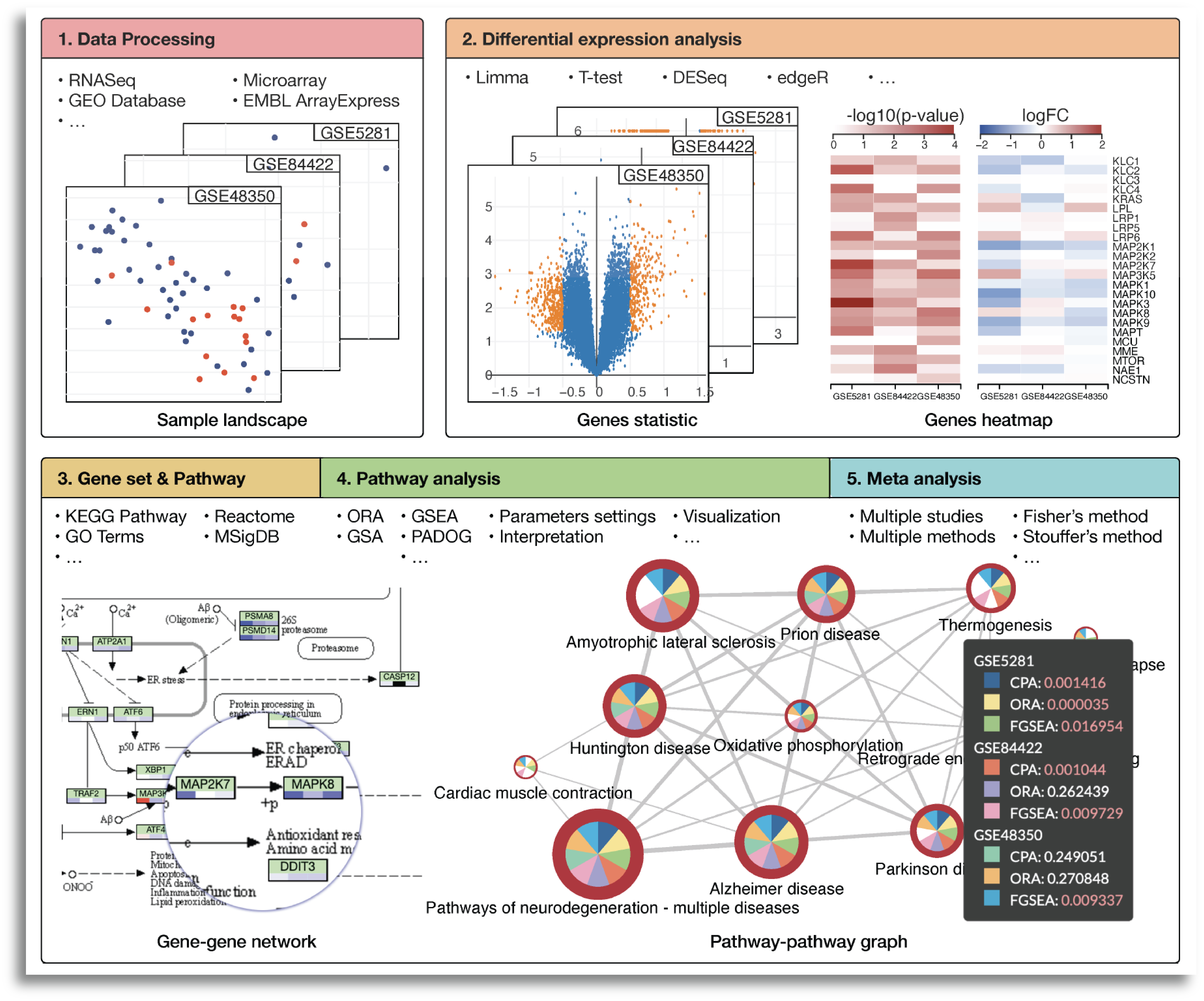
The course is structured such that the content will be arranged in five submodules which allows us to:
- Download and process data from public repositories,
- Perform differential analysis,
- Perform pathway analysis using different methods that seek to answer different research hypotheses,
- Perform meta-analysis and combine methods and datasets to find consensus results, and
- Interactively explore significantly impacted pathways across multiple analyses, and browsing relationships between pathways and genes.
- Getting Started
- Google Cloud Buckets
- Workflow Diagrams
- Google Cloud Architecture
- Software Requirements
- Data
- TroubleShooting
- Funding
- License
Each learning submodules will be organized in a R Jupyter notebook with step-by-step hands-on practice with R command line to install necessary tools, obtain data, perform analyses, visualize and interpret the results. The notebook will be executed in the Google Cloud environment. Therefore, the first step is to set up a virtual machine VertexAI.
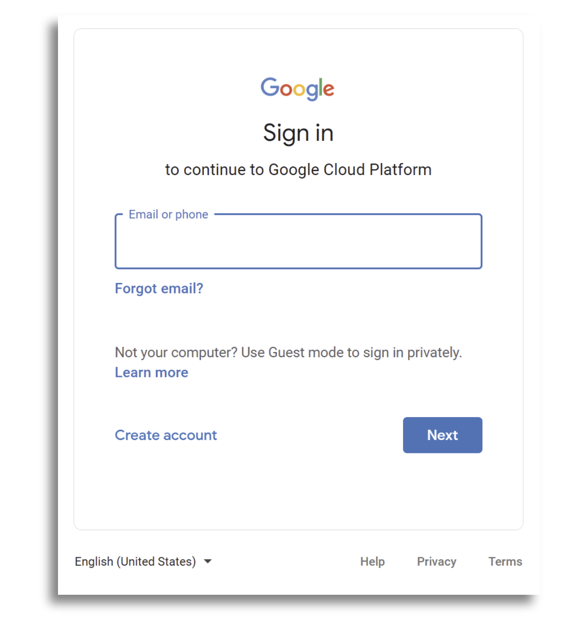
You can begin by first navigating to https://console.cloud.google.com/ and logging in with your credentials.
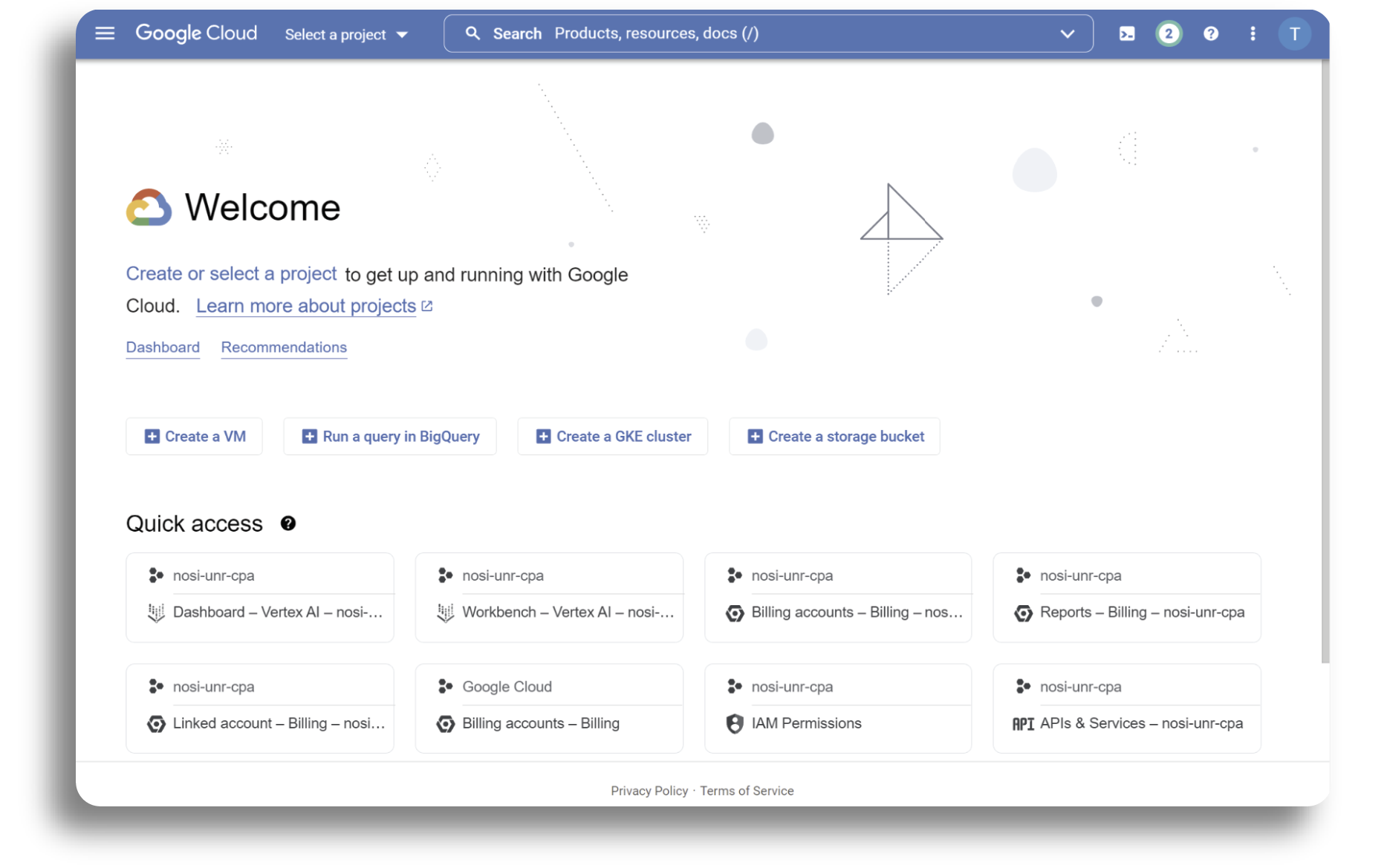
After a few moments, the GCP console opens with following dashboard.
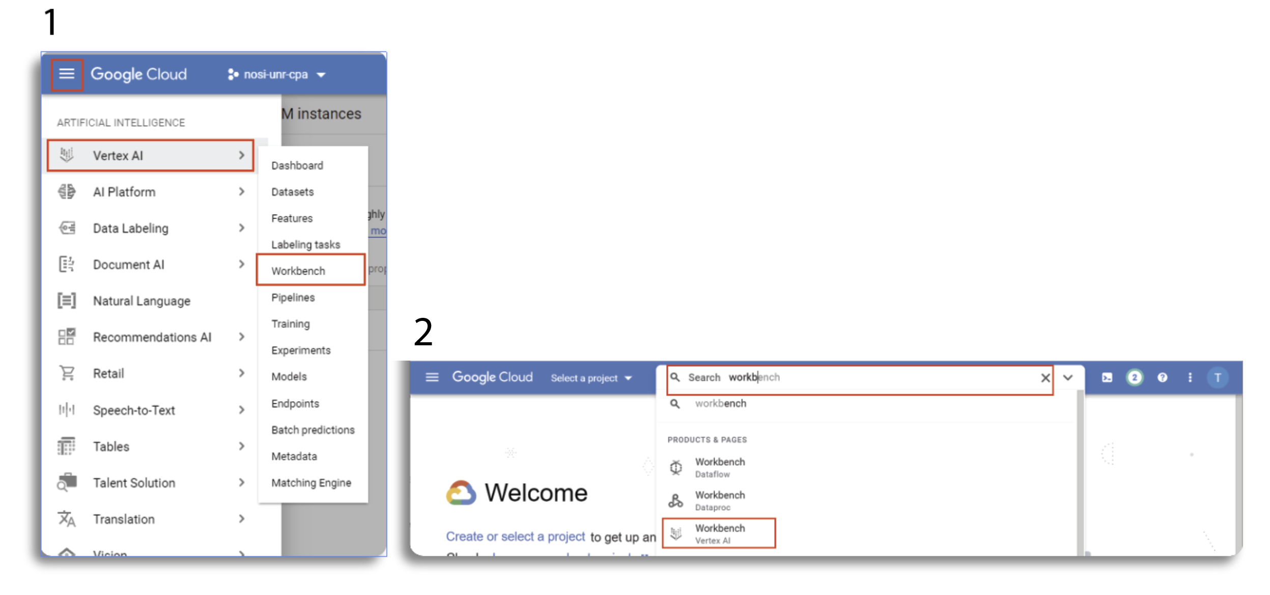
Once the login process is done, we can create a virtual machine for analysis using Vertex AI Workbench. There are two ways to navigate to Vertex AI. In the first method, we can click the Navigation menu at the top-left, next to “Google Cloud Platform”. Then, navigate to Vertex AI and select Workbench. In the second method, we can go to Google Cloud Console Menu in the Search products and resources, enter "Workbench" and then select Workbench Vertex AI.
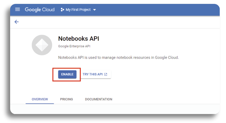
If it isn't already enabled we click Enable to start using the API.
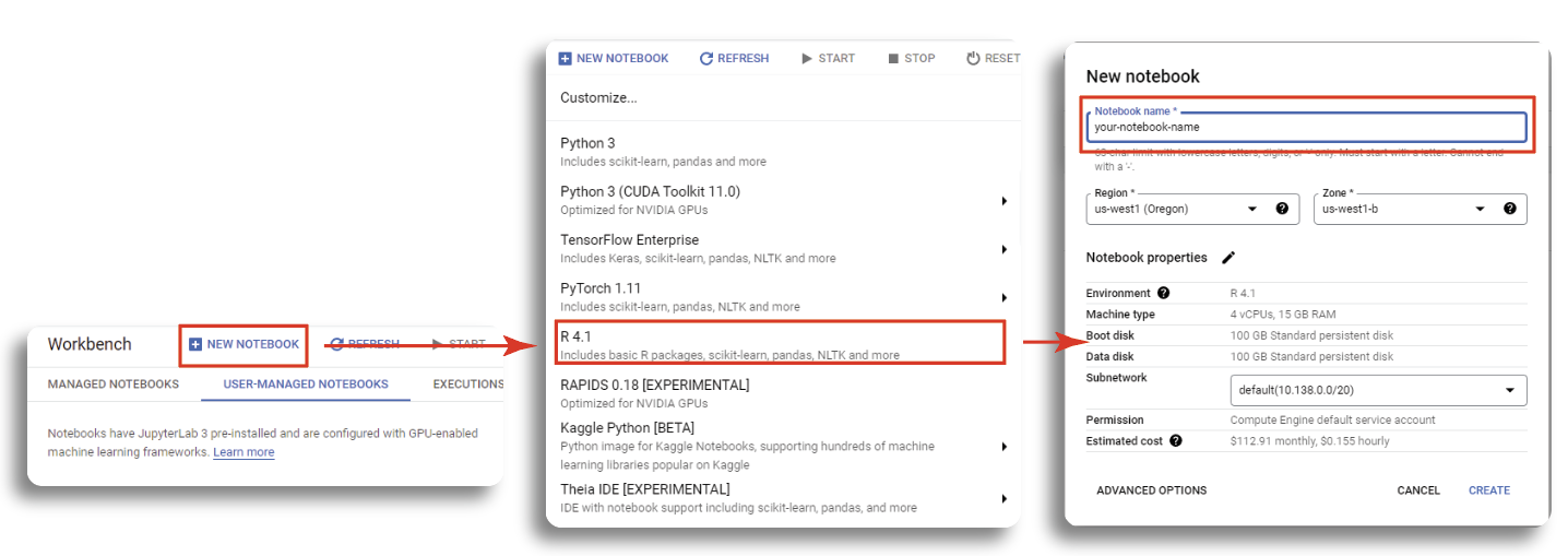
Within the Workbench screen, click MANAGED NOTEBOOKS, select the region which is closed to your physical location and click CREATE NOTEBOOK. Since our analyses will be based on R programing language, we need to select R 4.1 as our development environment. Then, set a name for your virutal machine and select the server which is closed to you physical location. In our learning module, a default machine with 4 vCPUS and 15GB RAM would be suffice. Finally, click CREATE to get the new machine up and running.
Creating a machine may take a few minutes to finish and you should see a new notebook with your designed name appears within the workbench dashboard when the process is completed.
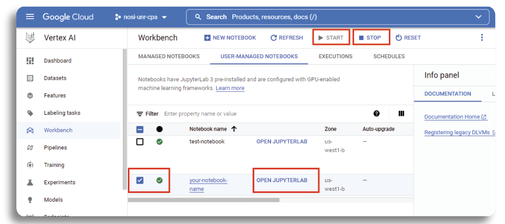
To start the virtual machine, select your notebook in the USER-MANAGED NOTESBOOK and click on START button on the top menu bar. The starting process might take up to several minutes. When it is done, the green checkmark indicates that your virtual machine is running. Next, clicking OPEN JUPYTER LAB to access the notebook.
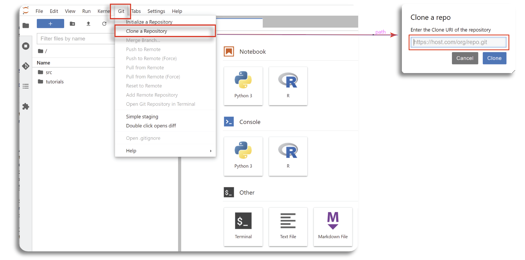
Now that you have successfully created your virtual machine, and you will be directed to Jupyterlab screen. The next step is to import our CPA's notebooks start the course. This can be done by selecting the Git from the top menu in Jupyterlab, and choosing the Clone a Repository option. Next you can copy and paste in the link of repository: "https://github.com/tinnlab/NOSI-Google-Cloud-Training.git" (without quotation marks) and click Clone.
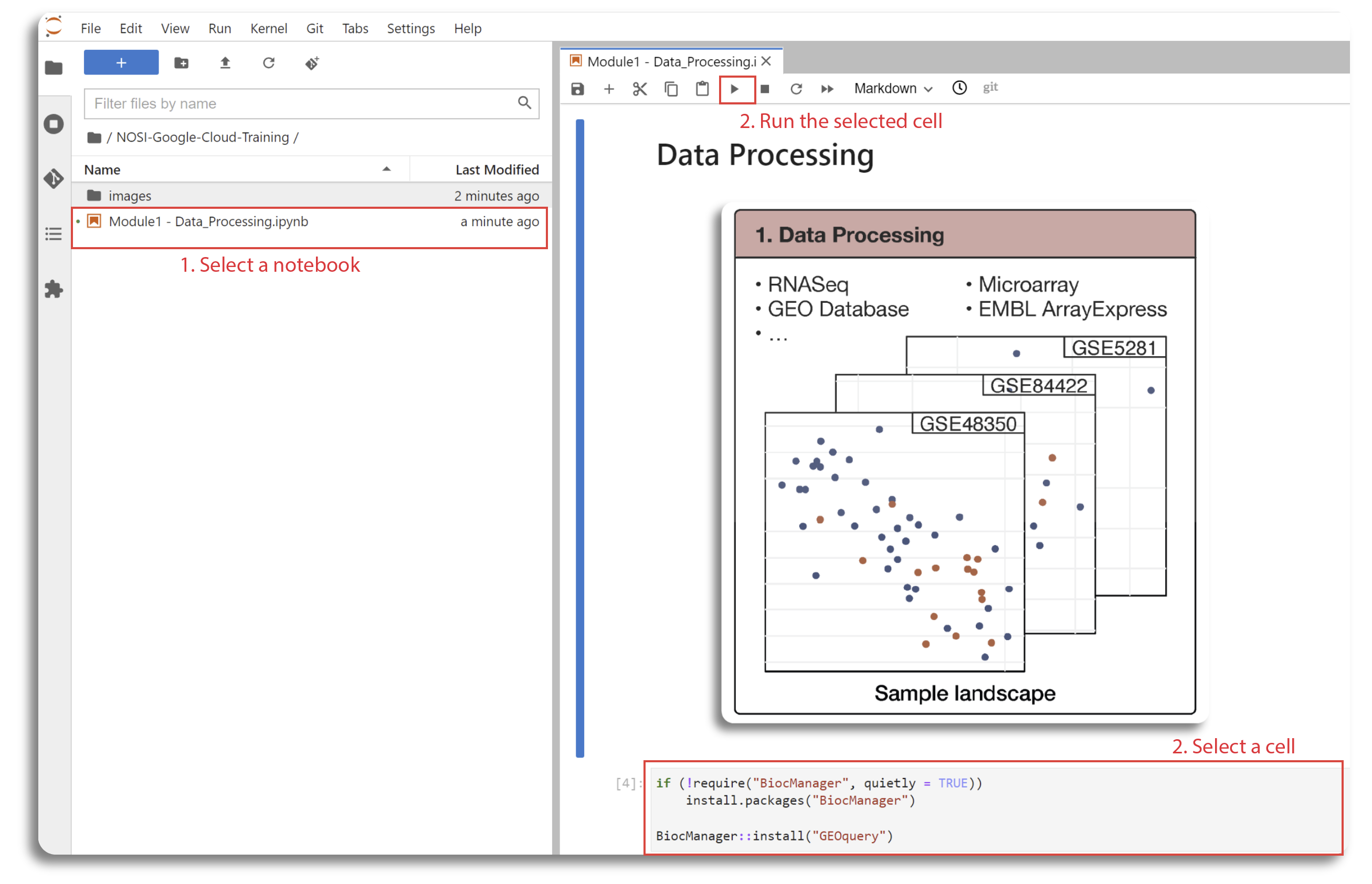
This should download our repository to Jupyterlab folder. All tutorial files for five sub-moudule are in Jupyter format with .ipynv extension . Double click on each file to view the lab content and running the code. This will open the Jupyter file in Jupyter notebook. From here you can run each section, or 'cell', of the code, one by one, by pushing the 'Play' button on the above menu.
Some 'cells' of code take longer for the computer to process than others. You will know a cell is running when a cell has an asterisk next to it [*]. When the cell finishes running, that asterisk will be replaced with a number which represents the order that cell was run in. You can now explore the tutorials by running the code in each, from top to bottom. Look at the 'workflows' section below for a short description of each tutorial.
Jupyter is a powerful tool, with many useful features. For more information on how to use Jupyter, we recommend searching for Jupyter tutorials and literature online.
When you are finished running code, you should turn off your virtual machine to prevent unneeded billing or resource use by checking your notebook and pushing the STOP button.
The content of the course is organized in R Jupyter Notebooks. Then we use Jupyter Book which is a package to combine individuals Jupyter Notebooks into a web-interface for a better navigation. Details of installing the tools and formatting the content can be found at: https://jupyterbook.org/en/stable/intro.html. The content of the course is reposed in the Github repository of Dr. Tin Nguyen's lab, and can be found at https://github.com/tinnlab/NOSI-Google-Cloud-Training. The overall structure of the modules is explained below:
- Submodule 01 describes how to obtain data from public repository, process
- and save the expression matrix and shows how to map probe IDs into gene symbols.
- Submodule 02 focuses on Differential Expression Analysis using
limma,t-test,edgeR, andDESeq2. - Submodule 03 introduces common curated biological databases such as Gene
- Ontology (GO), Kyoto Encyclopedia of Genes and Genomes (KEGG)
- Submodule 04 aims at performing Enrichment Analysis methods using popular
- methods such as
ORA,FGSEA, andGSA. - Submodule 05 aims at performing Meta-analysis using multiple datasets.
In this section, we will describe the steps to create Google Cloud Storage Buckets to store data generated during analysis. The bucket can be created via GUI or using the command line. To use the GUI, the user has to first visit https://console.cloud.google.com/storage/, sign in, click on Buckets on the left menu.
Next, click on the CREATE button below the search bar to start creating a new bucket.
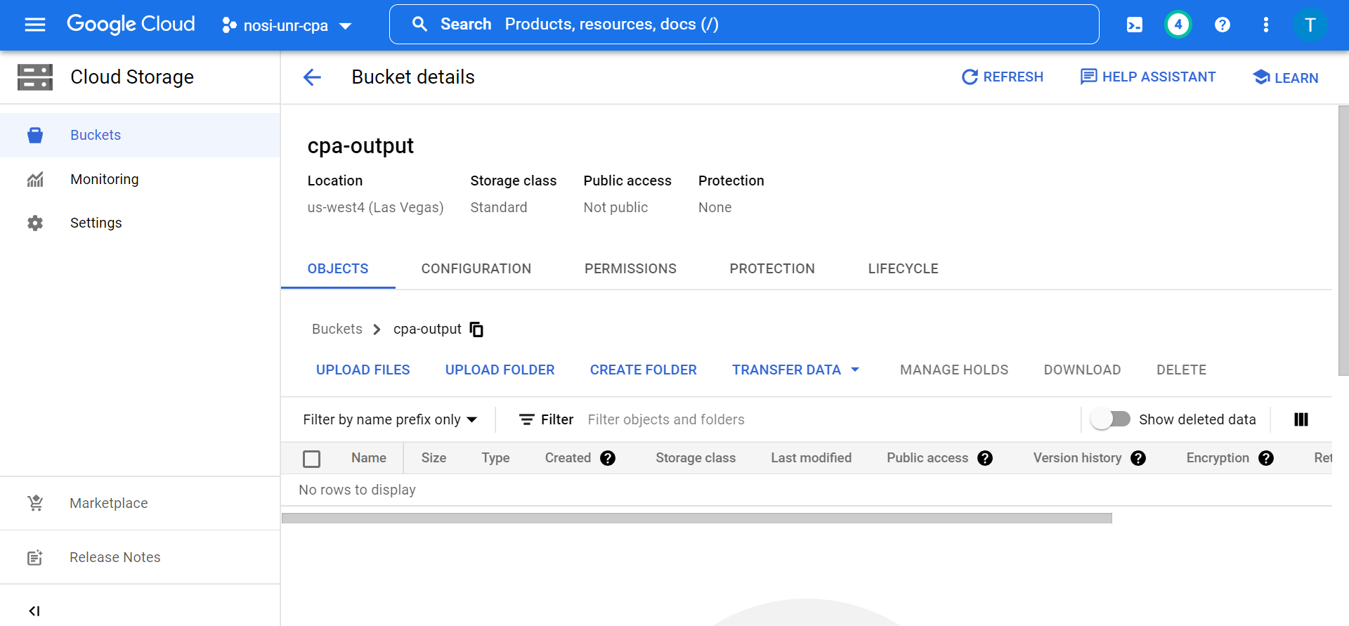
This will then open a page where the user will provide the unique name of the bucket, the location, access control and other information about the bucket. Here, we named our bucket as cpa-output. After this the user will click on the CREATE button to complete the process.
To create a Bucket using the command line, the user can use the gcloud storage buckets create command
gcloud storage buckets create gs://BUCKET_NAME where BUCKET_NAME is the user-defined name.
If the request succeeds, the user gets a success message. The user can also add optional flags
while running the create command to have greater control over the creation of the bucket.
Such flags include --project: PROJECT_NAME, --default-storage-class: STORAGE_CLASS, --location: LOCATION
and --uniform-bucket-level-access with PROJECT_NAME and STORAGE_CLASS supplied by the user.
Storage Buckets can also be created on the command line using the gsutils mb command.
The command to do so is gsutil mb gs://BUCKET_NAME, with BUCKET_NAME the desired bucket name.
This command also returns a success message upon completion and can also take optional flags
-p, -c, -l, -b and their user-supplied values, corresponding to project ID or number, default storage class,
location of the bucket and
uniform bucket-level access respectively, just like the create command.
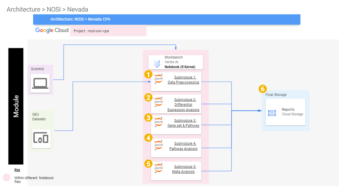
The figure above shows the architecture of the learning module with Google Cloud infrastructure. First, we will create an VertexAI workbench with R kernel. The code and instruction for each submodule is presented in a separate Jupyter Notebook. User can either upload the Notebooks to the VertexAI workbench or clone from the project repository. Then, users can execute the code directly in the Notebook. In our learning course, the submodule 01 will download data from the public repository (e.g. GEO database) for preprocessing and save the processed data to a local file in VertexAI workbench and to the user's Google Cloud Storage Bucket. The output of the submodule 01 will be used as inputs for all other submodules. The outputs of the submodules 02, 03, and 04 will be saved to local repository in VertexAI workbench and the code to copy them to the user's Cloud Bucket is also included.
This learning module does not require any computational hardware and local environment setting from users as the programs and scripts can be run in the browser-based development environment provided by Google. However, users need to have Google email account, sufficient internet access, and a standard web-browser (e.g. Chrome, Edge, Firefox etc., Chrome browser is recommended) to create a Cloud Virtual Machine for analysis. It is recommended to execute the Jupyter Note Book using R kernel version > 4.1 using a standard machine with minimum configuration of 4 vCPUs, 15 GB RAM, and 10GB of HDD.
All data from the modules were originally downloaded from the Gene Expression Omnibus (GEO) repository using the accession number GSE48350 file. The data was originally generated by Berchtold and Cotman, 2013. We preprocessed this data and normalized it, after which we used it in the subsequent analyses.
Some common errors include having the Jupyter Notebook kernel defaulting to Python and libraries not loading properly. To fix the kernel, check that the upper right hand corner of the edit ribbon says "R". If it doesn't, you can click the words next to the circle (O) to change the kernel. When there are problems loading a library, check that the package has been properly installed. Packages can usually be downloaded by the instructions in the documentation. Other errors that may happen are usually due to grammatical errors such as capitialization or spelling errors.
This work was fully supported by NIH NIGMS under grant number GM103440. Any opinions, findings, and conclusions, or recommendations expressed in this material are those of the authors and do not necessarily reflect the views of any of the funding agencies.
Text and materials are licensed under a Creative Commons CC-BY-NC-SA license. The license allows you to copy, remix and redistribute any of our publicly available materials, under the condition that you attribute the work (details in the license) and do not make profits from it. More information is available here.
This work is licensed under a Creative Commons Attribution-NonCommercial-ShareAlike 4.0 International License.
