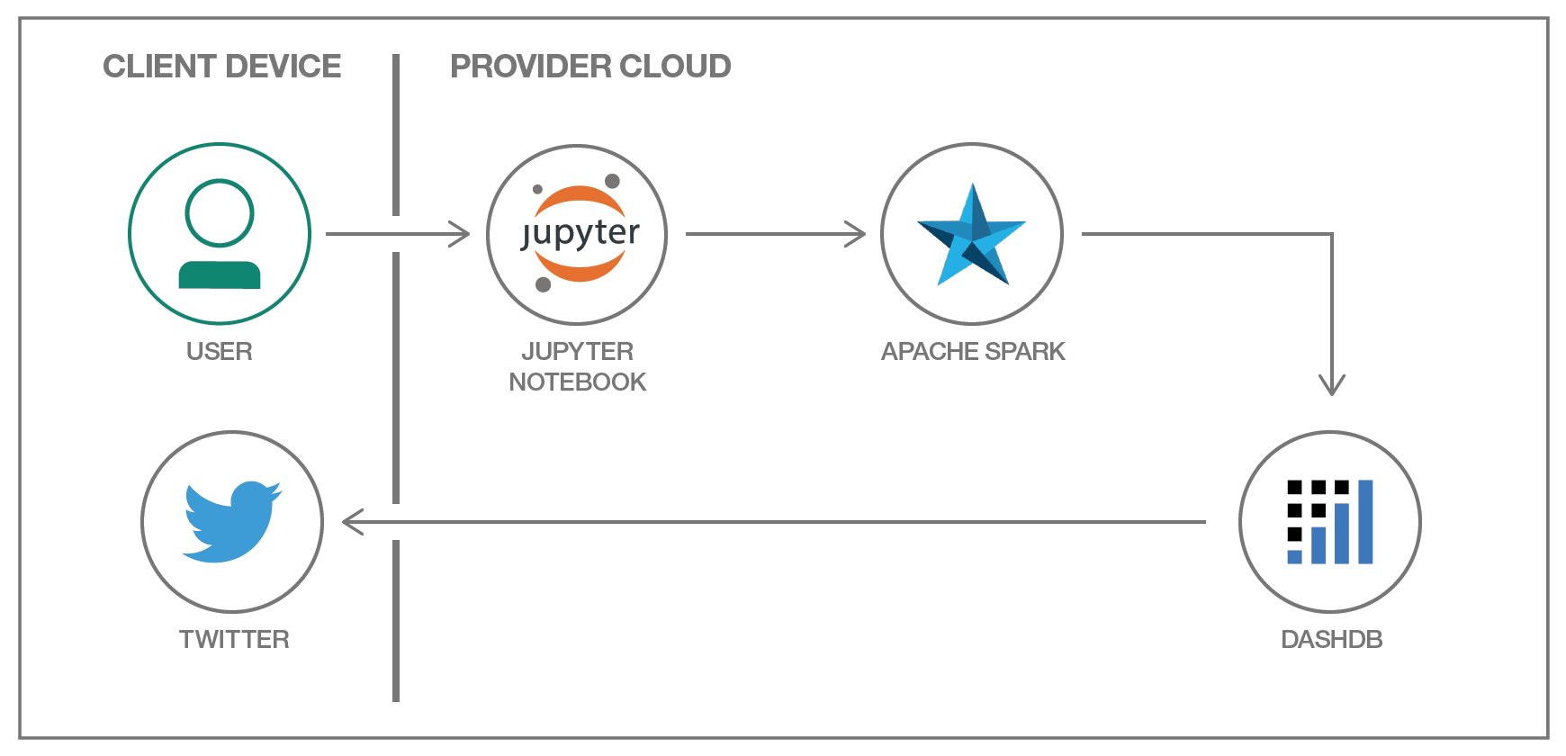
Twitter Analysis with Jupyter Notebooks

In this developer journey we will use Jupyter notebooks to analyze Twitter data and extract interesting insights from tweets. It will easily perform complex computations on a large amount of data in a notebook by using SparkContext, which enables you to run tasks on the Spark cluster. In addition, it will integrate data from dashDB using the Spark connector and use Spark and pandas DataFrames.

When the reader has completed this journey, they will understand how to:

Create a dashDB warehouse containing Twitter data that includes advanced enrichments like sentiment, gender and location.
Transform the data using Python code with Apache Spark and pandas data frames.
Create visualizations using Matplotlib and Google GeoChart.
Share notebooks and results.

The intended audience for this journey is application developers who need to efficiently build powerful data visualizations, but who may not have an abundance of time, data science experience or a dedicated data science team who could take ownership of such an effort.

Included Components

IBM Data Science Experience
Bluemix Insights for Twitter
Bluemix dashDB for Analytics
Bluemix Analytics for Apache Spark
Jupyter Notebooks
Python
pandas (Python Data Analysis Library)
NumPy
Wordcloud
Matplotlib
Google GeoChart

Steps

Follow these steps to setup and run this developer journey. The steps are described in detail below.

Sign up for the Data Science Experience
Create Bluemix services
Configure dashDB
Create the notebook
Run the notebook
Analyze the results
Save and Share

1. Sign up for the Data Science Experience

Sign up for IBM's Data Science Experience. By signing up for the Data Science Experience, two services: DSX-Spark and DSX-ObjectStore will be created in your Bluemix account.

2. Create Bluemix services

Create the following Bluemix services by clicking the Deploy to Bluemix button or by following the links to use the Bluemix UI and create them.

3. Configure dashDB

The first step in the analysis process is to harvest the Twitter data. In this sample, we use the dashDB connector to the IBM Insights for Twitter service to seamlessly specify a filter query (tweets about the six leading car manufacturers in 2015) and load the results into dashDB. This specific time frame and filter are being used to demonstrate analysis of a known Twitter spike.

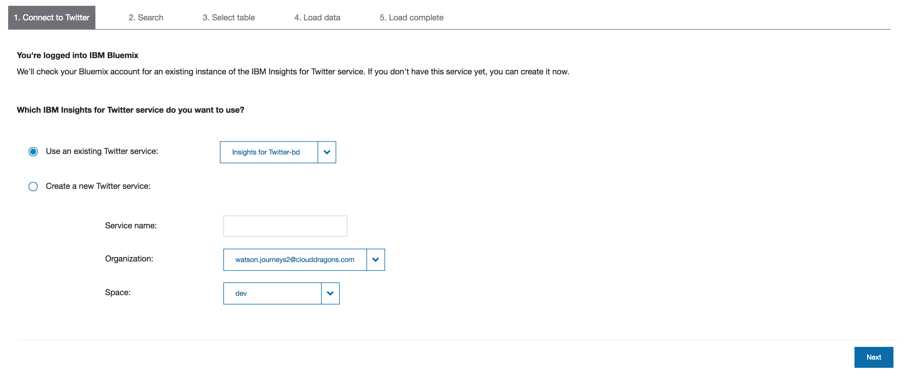
Launch the dashDB, from the menu on the left, choose Load and select Load Twitter Data. This is a five step process outlined below.
Connect to Twitter: Select the existing dashDB service you created earlier (if you used the Deploy to Bluemix button it is named "dtaa-dashdb-service").

Search: In the Search for Twitter data box, enter the query below and retrieve a sampling of tweets.

posted:2015-01-01,2015-12-31 followers_count:2000 listed_count:1000 (volkswagen OR vw OR toyota OR daimler OR mercedes OR bmw OR gm OR "general motors" OR tesla)

Select table: In the Load the data into new tables with this prefix field, enter any text you wish for a namespace.

Load data: This step can take up to 20 minutes, dashDB shows you progress as the tweets load.

Load complete: Peruse the reports that dashDB shows.

4. Create the notebook

Use the menu on the left to select My Projects and then Default Project. Click on Add notebooks (upper right) to create a notebook.

Select the From URL tab.
Enter a name for the notebook.
Optionally, enter a description for the notebook.
Enter this Notebook URL: https://github.com/IBM/dsx-twitter-auto-analysis/blob/master/notebooks/dsx_twitter_auto_analysis.ipynb
Use the Spark Service pulldown to select your DSX-Spark service.
Click the Create Notebook button.

5. Run the notebook

At the top of the notebook, provide your dashDB info.

Make sure you update SCHEMA and PREFIX with values you set when importing Twitter data into dashDB.
Use the username, password, and jdbcurl from the dashDB Service Credentials tab in BlueMix.

NOTE: You may have to create your own credentials using the New Credential option.

When a notebook is executed, what is actually happening is that each code cell in the notebook is executed, in order, from top to bottom.

Each code cell is selectable and is preceded by a tag in the left margin. The tag format is In [x]:. Depending on the state of the notebook, the x can be:

A blank, this indicates that the cell has never been executed.
A number, this number represents the relative order this code step was executed.
A *, this indicates that the cell is currently executing.

There are several ways to execute the code cells in your notebook:

One cell at a time.
- Select the cell, and then press the Play button in the toolbar.
Batch mode, in sequential order.
- From the Cell menu bar, there are several options available. For example, you can Run All cells in your notebook, or you can Run All Below, that will start executing from the first cell under the currently selected cell, and then continue executing all cells that follow.
At a scheduled time.
- Press the Schedule button located in the top right section of your notebook panel. Here you can schedule your notebook to be executed once at some future time, or repeatedly at your specified interval.

6. Analyze the results

The result of running the notebook is a report which may be shared with or without sharing the code. You can share the code for an audience that wants to see how you came your conclusions. The text, code and output/charts are combined in a single web page. For an audience that does not want to see the code, you can share a web page that only shows text and output/charts.

The charts produced in the journey clearly demonstrate the following:

There was a significant negative peak in tweets about car manufacturers during the period 2015-09-15 to 2015-10-15.

This spike was clearly dominated by tweets about the Volkswagen emissions scandal.

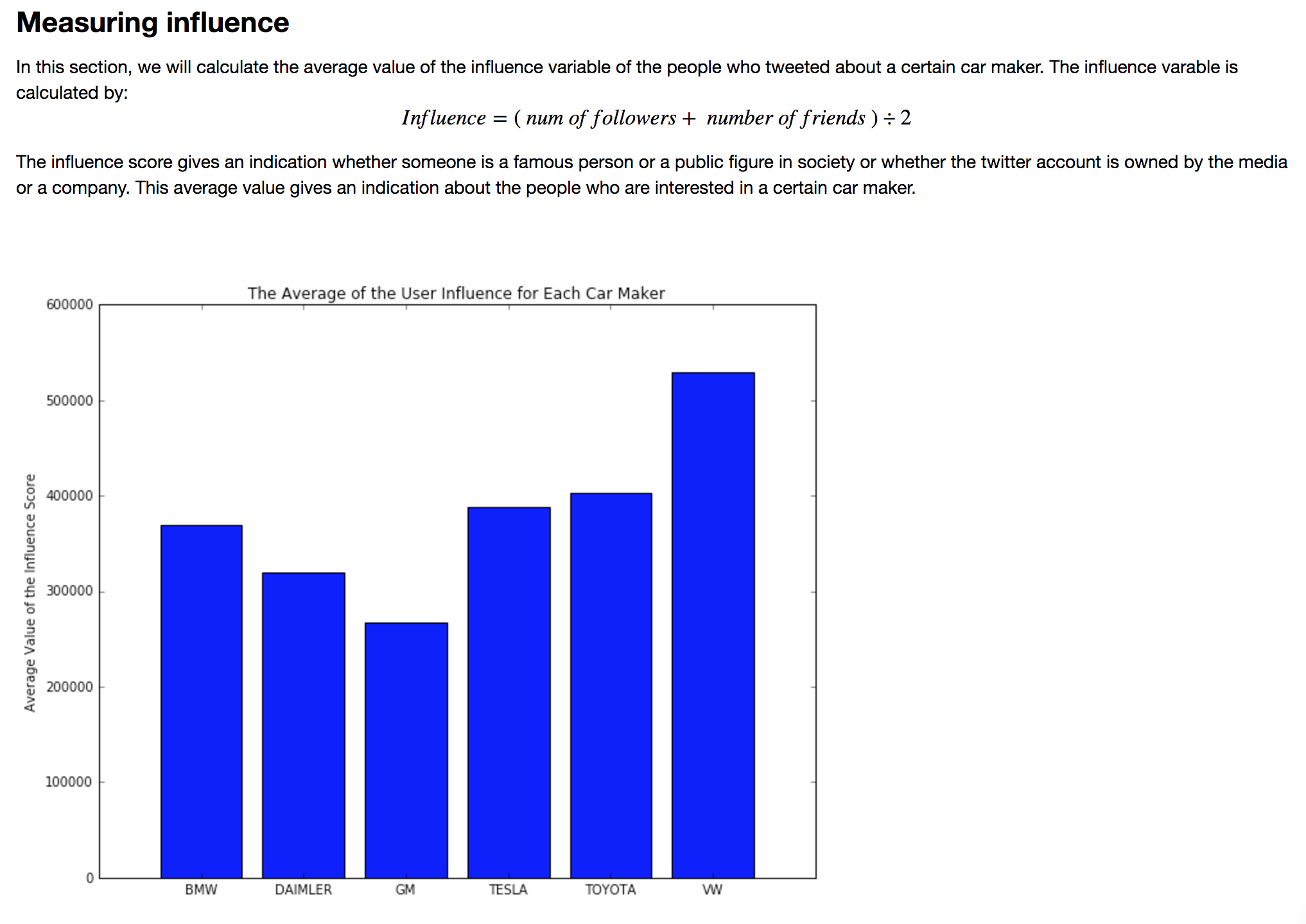
The amount of Twitter influence was slightly higher for Volkswagen than other car manufacturers.

The origin of the Volkswagen tweets was significantly from the United States and Europe.

The gender of the tweeters for Volkswagen (and all car makers) was significantly unknown. If we were to assume that the known-gender tweets are a good representative, then we could say predominantly male.

7. Save and Share

How to save your work:

Under the File menu, there are several ways to save your notebook:

Save will simply save the current state of your notebook, without any version information.
Save Version will save your current state of your notebook with a version tag that contains a date and time stamp. Up to 10 versions of your notebook can be saved, each one retrievable by selecting the Revert To Version menu item.

How to share your work:

You can share your notebook by selecting the “Share” button located in the top right section of your notebook panel. The end result of this action will be a URL link that will display a “read-only” version of your notebook. You have several options to specify exactly what you want shared from your notebook:

Only text and output: will remove all code cells from the notebook view.
All content excluding sensitive code cells: will remove any code cells that contain a sensitive tag. For example, # @hidden_cell is used to protect your dashDB credentials from being shared.
All content, including code: displays the notebook as is.
A variety of download as options are also available in the menu.

Sample output

The following is a sample data visualization with code:

For a full example without code see data/examples/sample_output.pdf.

Troubleshooting

See DEBUGGING.md.

License

Apache 2.0

tliakos/dsx-twitter-auto-analysis