electrostatics.py is a python module for electrostatics field and potential calculations, and field line and equipotential contour plots.
Install into python by executing
# pip install git+https://github.com/tomduck/electrostatics.git --user
Textbook examples are given below along with a selection of cases from the excellent paper "Electric field lines don't work" by Wolf, Van Hook and Weeks (Am. J. Phys., 64, 1996). Solid lines are the field lines, dotted lines are equipotential contours, and colours give the field strength.
In each case field lines are initialized symmetrically close to one (or more) charges. Paths are determined numerically from the streamline equation using an ODE solver. The integration parameters were adapted from Heiko Bauke's page on "Visualizing Streamlines".
The colours in each image give the logarithm of the field magnitude. Each colour step represents a 0.2 change in log-10 space (5 steps represents a decade). The field in close proximity to a charge is clipped to a maximum value.
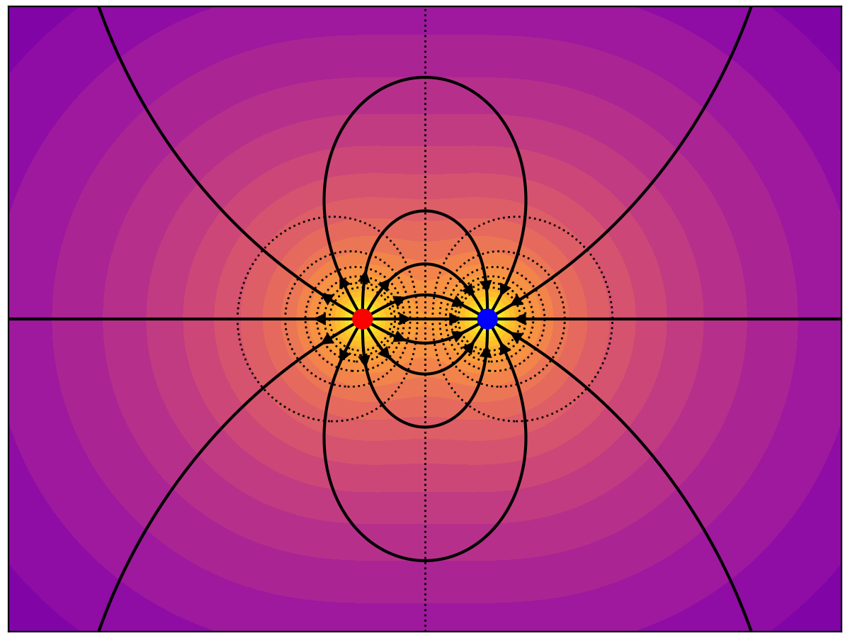
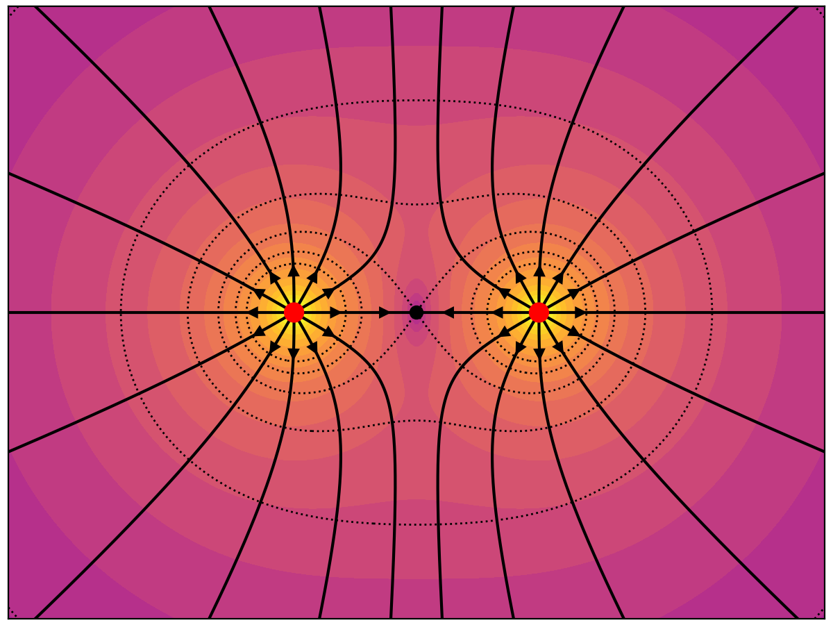
The left charge is +1 and the right charge is -1. In textbook examples like this the lines are symmetrically distributed around each charge no matter which charge they are initialized around.
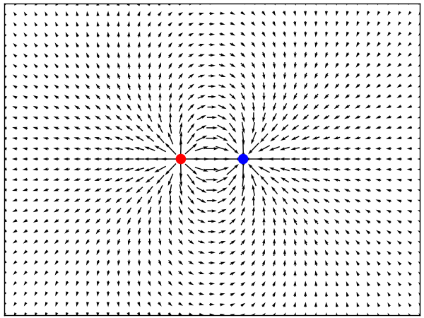
Below is the corresponding electric field vector plot. The length of the vectors is the fifth root of the electric field magnitude. The field line diagrams make visualizing the field much easier.
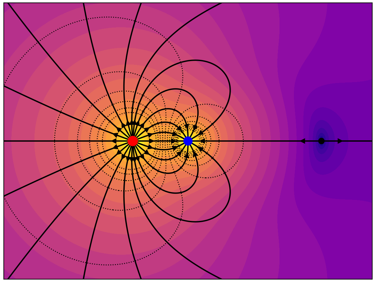
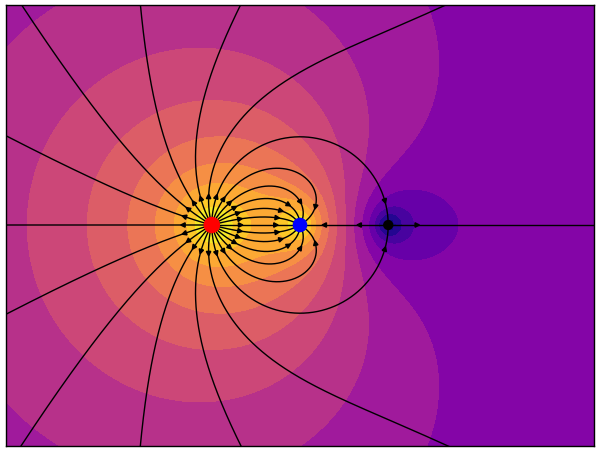
The left charge is +2 and the right charge -1. Field lines are initialized symmetrically around the -1 charge, and again symmetrically in the far field. Notice that the +2 charge exhibits "equatorial clumping" of the field lines, and that there is divergence from the zero-field point (in black). Equatorial clumping and 2D divergence are artefacts that arise from taking a 2D slice of a 3D field.
This example is for a theoretical electric field that is non-divergent in 2D (i.e., Flatland). There is no clumping and the zero-field point has the same number of lines entering and leaving it, as expected.
This is another textbook example. Note the equatorial clumping in the far field and the point of 2D convergence in the middle.
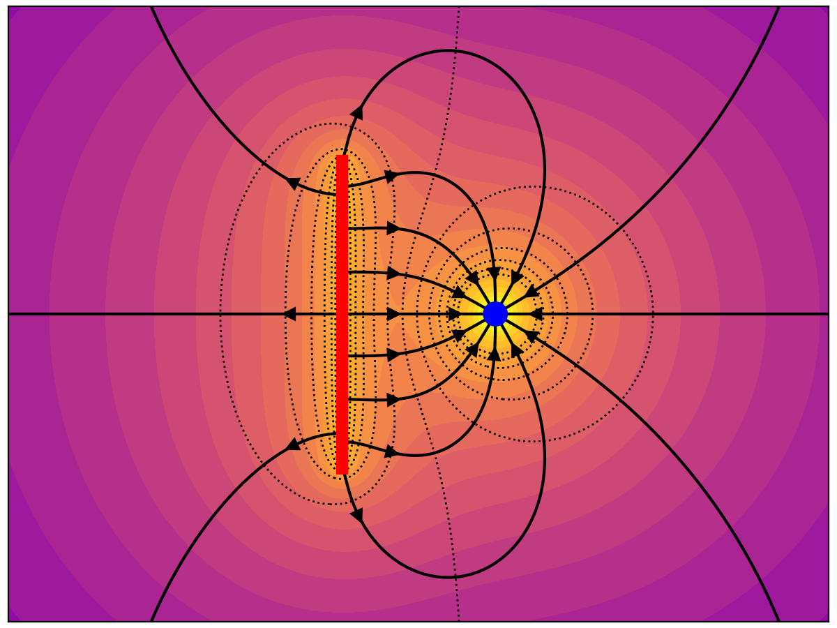
Both the line and point have the same amount of charge. Lines are initialized symmetrically around the point charge. That they do not connect to the line symmetrically is a 2D slice artefact.
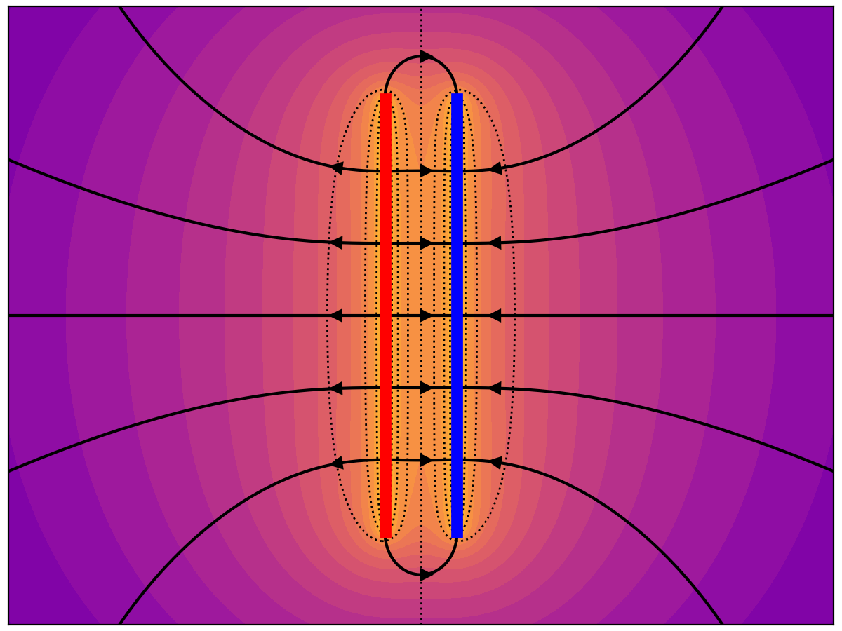
The lines are initialized symmetrically close to one line and connect to the other symmetrically, as expected.
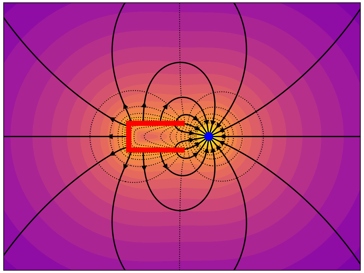
The cup and point have equal and opposite charges. Note that few field lines enter the cup.
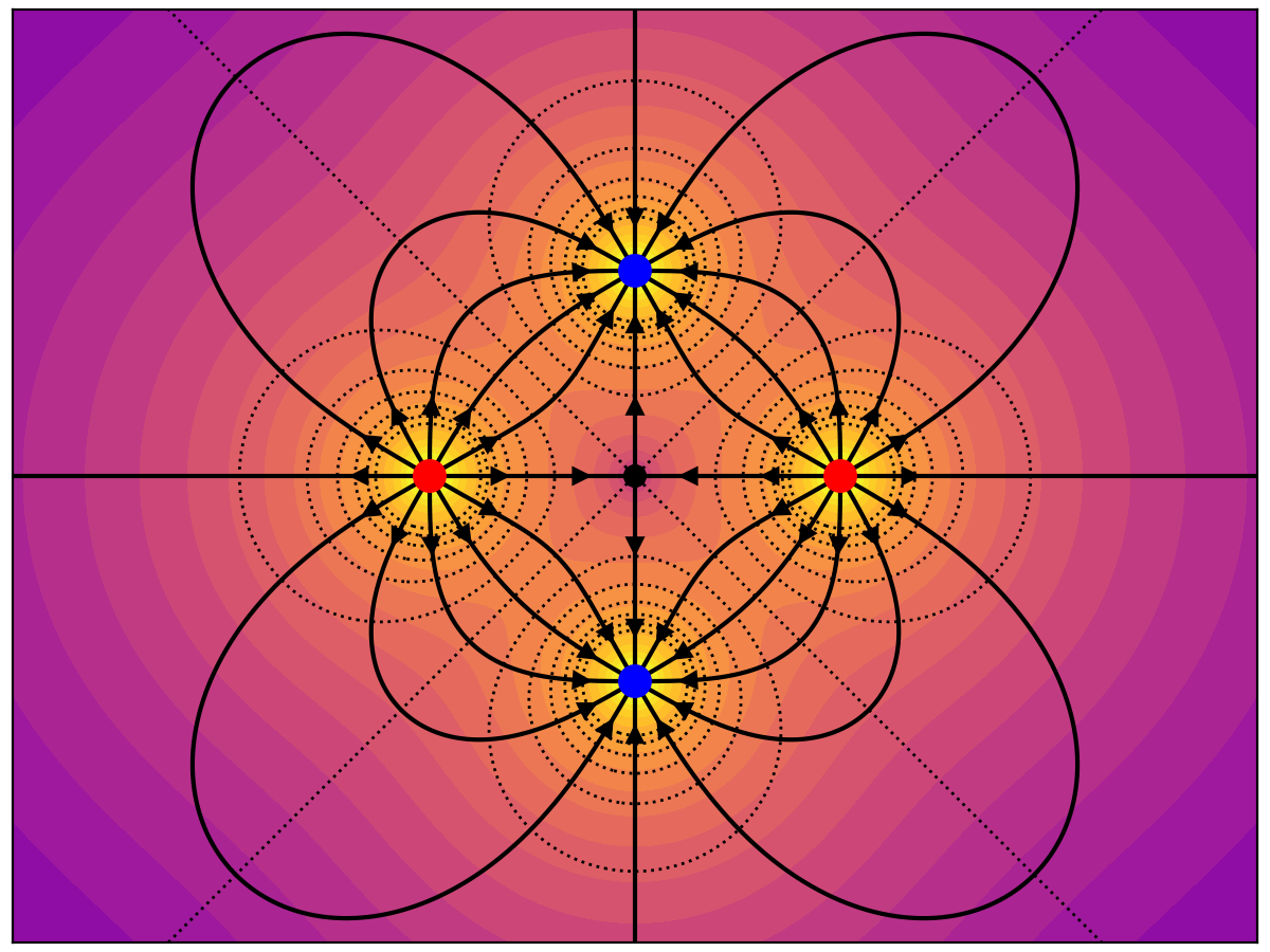
Another textbook example with perfect symmetry.
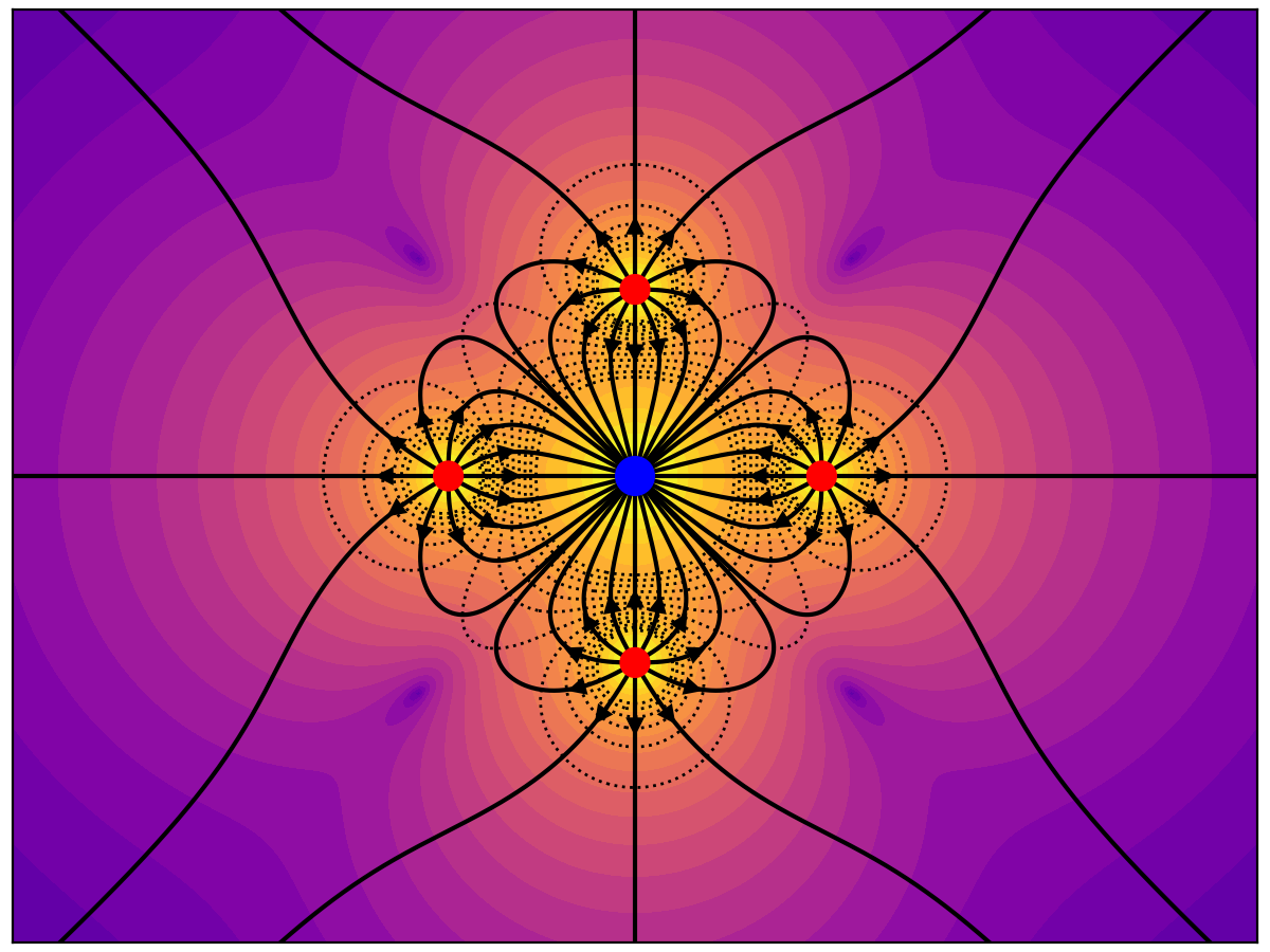
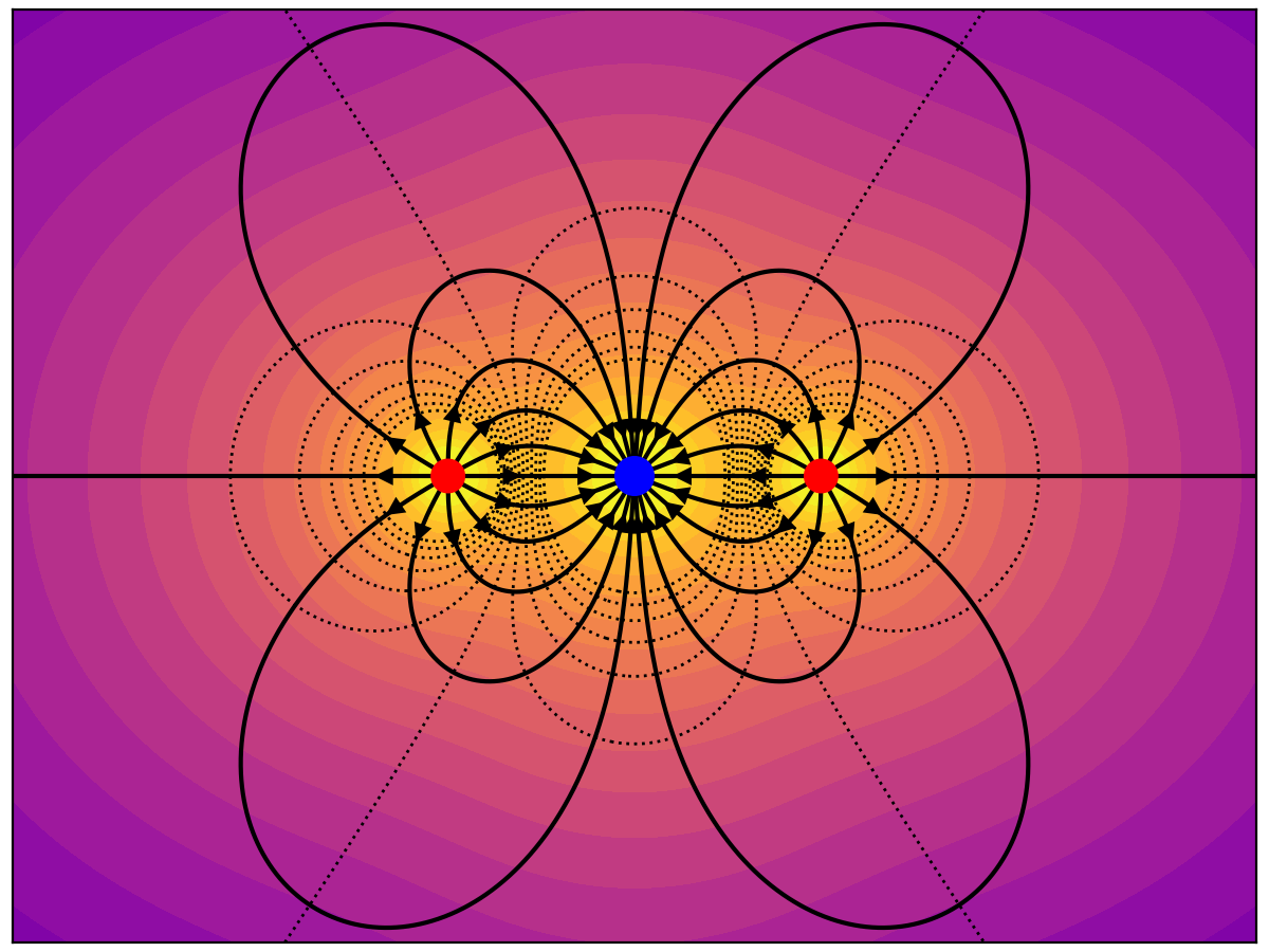
The middle charge is -4 and the outer charges are +2. Lines are initialized symmetrically around the positive charges. Note the equatorial clumping around the negative charge.
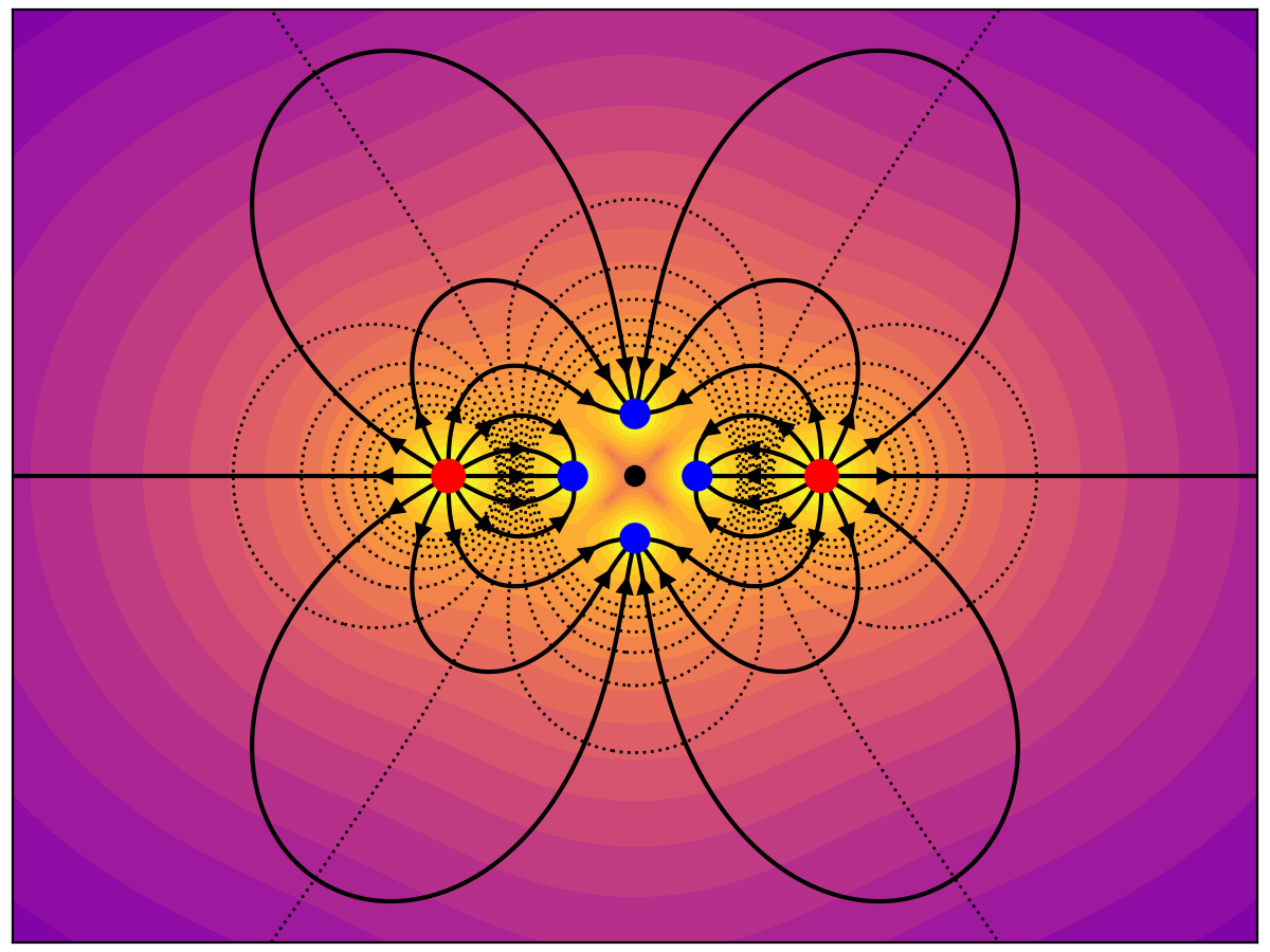
This is similar to the previous example but with the negative charge divided into a cluster of four -1 charges. Notice that there is an unequal distribution of lines between the negative charges. The number of lines is not proportional to the amount of charge in a 2D slice of a 3D field. The lines are also not distributed uniformly around the negative charges.
Here we have a -4 central charge surrounded by four +1 charges. 25% of the lines diverge to infinity, which incorrectly suggests a net +1 charge.