- 08/20/2019: Changed the default value of
lambdaparameter from 15 to 6 which is the value recommended by Engbert & Kliegl (2003). Note that there is no single generally correct or optimal value. When in doubt, compare different values oflambdaand see what works best for your data and application. - 03/15/2019: New features:
- Heuristics for blink and artifact detection.
- More options for the function producing diagnostic plots.
- Fixed a small bug in the saccade detection which made fixation durations one sample shorter than they should be.
- More robust estimates of fixation position and dispersion (using median and median absolute deviation).
- Easier installation directly from GitHub.
- 02/16/2015:
saccadesis now available on CRAN.
An R package for detection of saccades, fixations, and blinks in eyetracking data. It uses the velocity-based algorithm for saccade detection proposed by Ralf Engbert and Reinhold Kliegl (Vision Research, 2003). Any period occurring between two saccades is considered to be a fixation or a blink. Blink detection is done with a simple heuristic (when the spatial dispersion is close to zero, it’s likely a blink). Anything that doesn’t look like a saccade, fixation, or blink, is categorized as one out of multiple types of artifacts.
The package is available on CRAN. The latest version can be installed from GitHub using the following commands:
library("devtools")
install_github("tmalsburg/saccades/saccades", dependencies=TRUE)
Note that this package depends on the R package zoom which will be automatically installed with the commands above.
library(saccades)
data(samples)
fixations <- subset(detect.fixations(samples), event=="fixation")
head(fixations)
trial start end x y mad.x mad.y peak.vx peak.vy dur event 0 1 0 79 53.720 377.250 0.770952 1.275036 1.565 1.565 79 fixation 1 1 92 280 39.640 379.090 1.082298 0.859908 -2.125 -1.530 188 fixation 2 1 292 385 60.125 380.165 1.734642 0.822843 2.420 1.700 93 fixation 3 1 439 577 18.810 58.620 1.423296 1.660512 -1.205 2.310 138 fixation 4 1 606 1594 40.235 38.620 2.157183 2.149770 2.795 -2.740 988 fixation 5 1 1602 2916 47.265 35.300 1.964445 1.393644 -2.770 0.965 1314 fixation
The package contains sample eye movement data that was collected with an SMI IViewX system recording at 240Hz. The data set was deliberately chosen to have poor quality with periods of track loss and other issues. The data can therefore be used to investigate the various failure modes of the algorithm.
The data set contains for each sample, it’s x- and y-coordinate (in pixels on the screen), the time at which it was recorded (in ms), and the trial in which it was recorded. The samples on the coordinates (0,0) represent track loss.
library(saccades)
data(samples)
head(samples)
Loading required package: zoom time x y trial 1 0 53.18 375.73 1 2 4 53.20 375.79 1 3 8 53.35 376.14 1 4 12 53.92 376.39 1 5 16 54.14 376.52 1 6 20 54.46 376.74 1
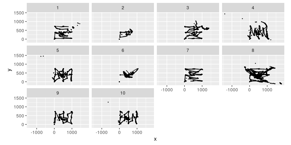
A plot showing the raw samples of the 10 trials:
library(tidyverse)

ggplot(samples, aes(x, y)) +
  geom_point(size=0.2) +
  coord_fixed() +
facet_wrap(~trial)The function detect.fixations detects eye movement events during which the eyes were stationary. These are primarily fixations, but also include blinks and artifacts (false positives produced by the velocity-based algorithm).
fixations <- detect.fixations(samples)
head(fixations)
trial start end x y mad.x mad.y peak.vx peak.vy dur event 0 1 0 79 53.720 377.250 0.770952 1.275036 1.565 1.565 79 fixation 1 1 92 280 39.640 379.090 1.082298 0.859908 -2.125 -1.530 188 fixation 2 1 292 385 60.125 380.165 1.734642 0.822843 2.420 1.700 93 fixation 3 1 439 577 18.810 58.620 1.423296 1.660512 -1.205 2.310 138 fixation 4 1 606 1594 40.235 38.620 2.157183 2.149770 2.795 -2.740 988 fixation 5 1 1602 2916 47.265 35.300 1.964445 1.393644 -2.770 0.965 1314 fixation
In the data frame returned by detect.fixations, each event is represented by a line. The columns are:
trial- the trial id
start,end- start and end time of the event
x,y- position of the event, estimated as the median coordinates of the samples that make up this event
mad.x,mad.y- spatial dispersion of the samples that make up this event, measured as the median absolute deviation of the x- and y-coordinates of the samples
peak.vx,peak.vy- peak horizontal and vertical velocity measured as differences between two consecutive samples
dur- the duration of the event
event- the type of event: fixation, blink, and artifacts too dispersed and too short
The results of the saccade detection can be examined visually using the function diagnostic.plot:
diagnostic.plot(samples, fixations)Called as above, the function will open an interactive plot showing the original samples and the detected fixations. The complete data set can be navigated using the mouse or keyboard (keyboard shortcuts shown in the console).
Non-interactive plots can be produced by setting the parameter interactive to FALSE. Additional arguments (e.g., ylim are passed through to the plot function.
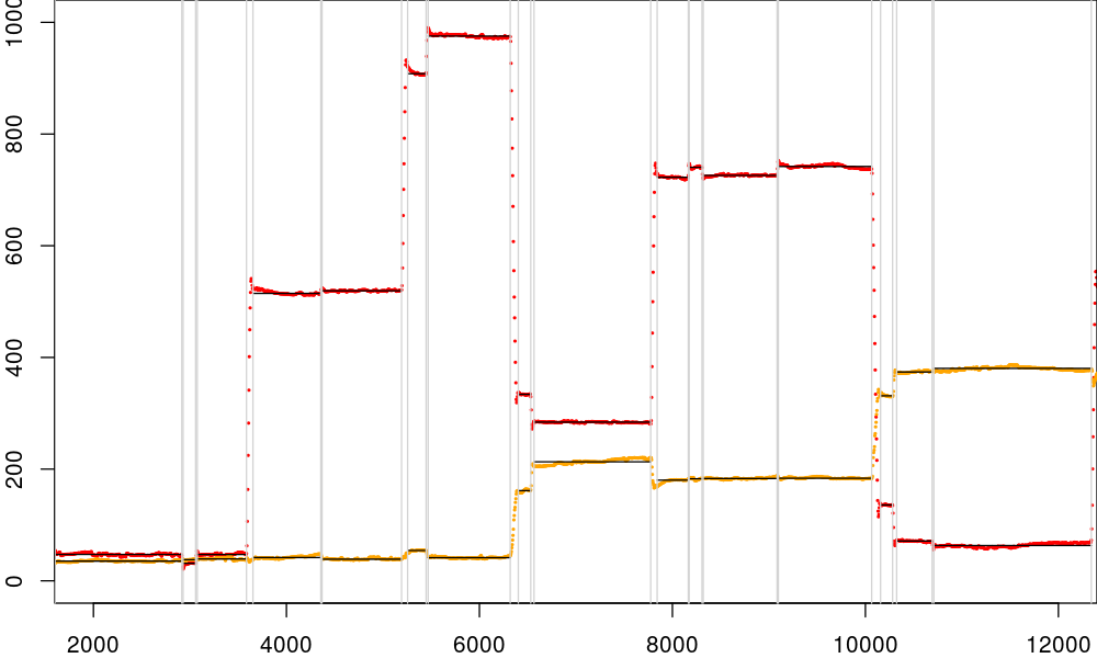
diagnostic.plot(samples, fixations, start.time=2000, duration=10000, interactive=FALSE, ylim=c(0,1000))The dots are the raw samples. Red dots represent the x-coordinate and orange the y-coordinate. The vertical lines mark the on- and offsets of fixations. The horizontal lines (difficult to see in the plot above) represent the fixations.
The function calculate.summary prints some summary statistics about the detected fixations:
stats <- calculate.summary(fixations)
round(stats, digits=2)
mean sd Number of trials 10.00 NA Duration of trials 37029.30 16508.56 No. of fixations per trial 107.30 50.86 Duration of fixations 314.67 443.14 Dispersion horizontal 5.42 53.84 Dispersion vertical 4.00 33.19 Peak velocity horizontal 3.58 133.23 Peak velocity vertical 1.05 88.62
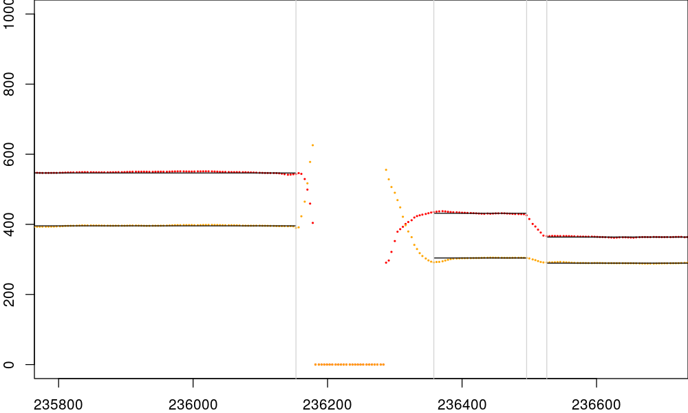
Blinks are fairly easy to spot (see graph below). It starts with something that looks like a saccade, then there’s a fixation on the coordinates (0,0) and with zero dispersion, and then there’s another saccade. In this data set samples on coordinates (0,0) indicate track loss. In data from EyeLink systems, 1e+08 is used for track loss. So the heuristic for blinks used in this package is: anything that looks like a fixation but has much lower dispersion than the typical fixation. Specifically, a blink is an event with a dispersion that is smaller than the median dispersion minus four times the median absolute deviation of the dispersion and only if this is the case for horizontal and vertical dispersion.
diagnostic.plot(samples, fixations, start.time=235800, duration=900, interactive=FALSE, ylim=c(0,1000))Other non-fixation events are artifacts. The most common type are spurious micro fixations that are detected between the main sweep of the saccade and the swing back (a.k.a. glissade or j-hook) at the end of saccades. During this time the velocity momentarily drops below the threshold for saccade detection which results in the detection of an event. This is particularly likely to happen in high-frequency data, i.e. 1KHz and more but can also happen at lower frequencies. These artifacts are detected when the duration of the event is at least five median absolute deviations shorter than the median of all events.
Another type of artifact are events with a dispersion that is at least four median absolute deviations higher than the median dispersion. These tend to happen rarely and primarily with very low quality data.
The default setting work well with high-frequency data from current research-grade eye-trackers such as SMI’s IViewX system and SR Research’s EyeLink system. Playing with the parameters can make sense when the data is low quality (noisy, excessive track loss) or sampled at frequencies below (200Hz). The following parameters can be changed:
lambda- specifies which multiple of the standard deviation of the velocity distribution should be used as the detection threshold. The default setting of 6 is recommended in Engbert & Kliegl (Vision Research, 2003).
smooth.coordinates- logical indicating whether x- and y-coordinates should be smoothed using a moving average with window size 3 prior to saccade detection. Can be useful when the data is very noisy (low precision). With high-quality data setting this to true hurts more than it helps because it slightly lowers the precision of the on- and off-sets of events.
smooth.saccades- logical. If
TRUE, consecutive saccades separated by only one sample will be joined. This can avoid detection of micro fixations before swing-backs. Whether this works well, depends on the sampling rate of the eye-tracker. If it’s high, say higher than 500Hz, most gaps between the main sweep and the swing-back become too large to be affected by this setting. Similarly this setting discards one-sample saccades. Note that when the data is low-frequency this can have the consequence that most or even all saccades are discarded.
Yes. The quality of saccade and fixation detection is going to be lower than with higher frequency data, but in my experience the results can, with some tweaking, still be better than those produced by manufacturer-supplied algorithms. Note, though, that the default settings are optimized for use with data recorded at frequencies above 200Hz. When working with data from cheaper and slower eye-trackers, it can make sense to set smooth.coordinates to TRUE (to suppress noise) and to set smooth.saccades to FALSE (to detect short saccades more reliably). Playing with the lambda parameter can also help.


